bqplot - Interactive Plotting in Jupyter Notebook | Python
Bqplot is an interactive data visualization library of Python developed by researchers at Bloomberg. The library is built on top of java script and Python library ipywidgets.
The main aim of bqplot is to bring in benefits of javascript functionality to python along with utilizing widgets facility of ipywidgets by keeping all chart components as widgets to infuse flexibility.
All of the individual components of the graph in bqplot are interactive widgets based on ipywidgets. This gives a lot of flexibility with regard to creating interactive visualization as well as easy integration with other notebook widgets.
What Can You Learn From This Article?
As a part of this tutorial, we have explained how to create interactive charts in jupyter notebook using Python library bqplot. We'll be using pyplot API of bqplot which is same as pyplot API of matplotlib to create various data visualizations. Tutorial covers many different chart types like scatter charts, bar charts, line charts, and many more. Apart from creation of charts, tutorial explains how to improve chart aesthetics. Tutorial is a good starting point for someone who is new to bqplot and wants to learn it properly.
Two Different APIs Of Bqplot to Create Charts
Bqplot provides 2 kinds of APIs for creating plots:
Matplotlib pyplot-like API: It provides the same set of functions as that available in "matplotlib.pyplot" module. We can easily create graphs by calling methods like scatter(), bar(), pie(), heatmap(), etc.
Internal object model API: It provides API which lets us create an object for each individual graph component like figure, axis, scales, etc. Each of these objects behaves as a widget and can be linked to other widgets. We need to then combine all of this to create a plot. This API gives more flexibility.
We'll be concentrating on pyplot API in this tutorial. If you have a background with matplotlib then this tutorial will be a smooth ride for you.
If you are interested in learning about plotting with internal object model API then please feel free to visit our tutorial on it:
Important Sections Of Tutorial
- Load Datasets
- Wine Dataset
- Apple OHLC Dataset
- World Happiness Dataset
- Scatter Plots
- Bar Charts
- Grouped Bar Chart
- Stacked Bar Chart
- Line Charts
- Histograms
- Pie Charts (Donut Charts)
- BoxPlots
- HeatMaps
- Candlestick Charts
- Choropleth Maps
Bqplot Video Tutorial
Please feel free to check below video tutorial if feel comfortable learning through videos. We have covered three different chart types in video. But in this tutorial, we have covered many different chart types.
Below, we have imported bqplot and printed the version of it that we have used in our tutorial.
import bqplot

print("Bqplot Version : {}".format(bqplot.__version__))
import warnings
warnings.filterwarnings("ignore")
Load Datasets
We'll be loading all datasets from the beginning and will be keeping them as pandas dataframe to make plotting easy.
1. Wine Dataset
The first dataset that we'll be loading is wine dataset available with scikit-learn. It has information about wine ingredients and their presence in three different wine categories.
import pandas as pd
from sklearn.datasets import load_wine

wine  = load_wine()

print("Dataset Features : ", wine.feature_names)
print("Dataset Size : ", wine.data.shape)

wine_df = pd.DataFrame(data=wine.data, columns=wine.feature_names)
wine_df["Category"] = wine.target

wine_df.head()
2. Apple OHLC Data from Yahoo Finance
Another dataset that we'll be using for our explanation purpose is APPLE OHLC data downloaded from yahoo finance as CSV. We'll be loading it as a pandas dataframe.
import pandas as pd

apple_df = pd.read_csv("~/datasets/AAPL.csv", index_col=0, parse_dates=True)

apple_df.head()
3. World Happiness Dataset
The third dataset that we'll be using for an explanation of map charts is world happiness dataset available on kaggle.
It has information about attributes like happiness score, perception of corruption, healthy life expectancy, social support by govt., freedom to make life choices, generosity and GDP per capita for various countries of the earth.
We'll be loading it as a pandas dataframe.
import pandas as pd

happiness_df = pd.read_csv("~/datasets/world_happiness_2019.csv")

happiness_df.head()
We suggest that you download all datasets beforehand and keep it in the same directory as a jupyter notebook to follow along with a tutorial. We'll now start by plotting various plots to explain the usage of bqplot's pyplot API.
1. Scatter Plots 
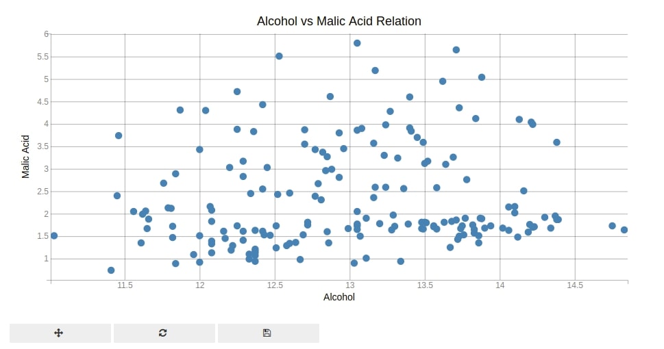
The first plot type that we'll introduce is a scatter plot. We'll plot the alcohol vs malic acid relationship using a scatter plot.
Below, We have first created a figure. Then, we have created a scatter plot using scatter() method of pyplot. We have given alcohol values to x parameter and malic acid values to y parameter.
Then, we have set X and Y axes labels.
At last, we have called show() method to display chart.
from bqplot import pyplot as plt

fig = plt.figure(title="Alcohol vs Malic Acid Relation")

scat = plt.scatter(x=wine_df["alcohol"], y=wine_df["malic_acid"])

plt.xlabel("Alcohol")
plt.ylabel("Malic Acid")

plt.show()
NOTE
Please make a note that all the charts won't be interactive on web-page here but when you run it in a jupyter notebook then they'll be interactive.
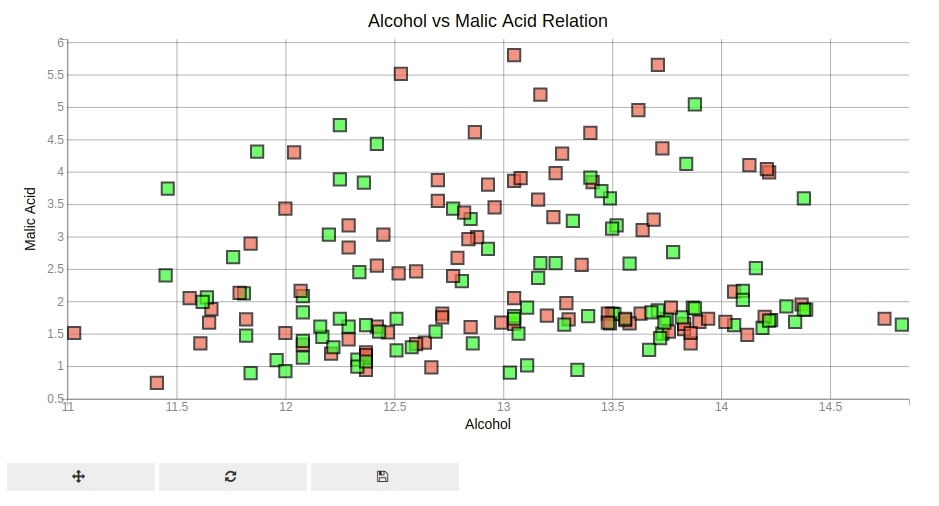
Below we are trying to modify scatter plot by passing arguments related to color, edge color, edge width, marker size, market type, opacity, etc.
Below we have explained another way of setting axis attributes by passing them as a dictionary to the axes_options parameter. We need to use stroke and stroke_width parameters to modify the line property of markers. We have used square markers for this scatter plot and 2 different colors to color individual markers.
from bqplot import pyplot as plt

fig = plt.figure(title="Alcohol vs Malic Acid Relation", )

options = {'x':{'label':"Alcohol"}, 'y':{'label':'Malic Acid'}}

scat = plt.scatter(wine_df["alcohol"], wine_df["malic_acid"],
                   colors=["lime", "tomato"],
                   axes_options = options,
                   stroke="black", stroke_width=2.0,
                   default_size=150,
                   default_opacities=[0.7],
                   marker="square",
                   )

plt.show()
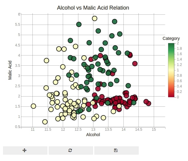
We can even access the layout object from the figure object and then modify plot width and height by setting their values as pixels.
We are also setting the x-axis label, y-axis label and x-axis limit to further enhance the graph.
We are also color-encoding points according to the wine category. We also have changed the color bar location through the axes_options parameter. We are color-encoding points of scatter plot by using different wine categories.
from bqplot import pyplot as plt

fig = plt.figure(title="Alcohol vs Malic Acid Relation")

fig.layout.height = "500px"
fig.layout.width = "600px"

options = {'color': dict(label='Category', orientation='vertical', side='right')}

scat = plt.scatter(x = wine_df["alcohol"], y = wine_df["malic_acid"],
                   color=wine_df["Category"],
                   axes_options = options,
                   stroke="black", stroke_width=2.0,
                   default_size=200,
                   default_opacities=[0.9],
                   marker="circle",
                   )

plt.xlabel("Alcohol")
plt.ylabel("Malic Acid")

plt.xlim(10.7, 15.3)

plt.show()
Below we are introducing tooltip which will highlight Wine Category, Alcohol and Malic Acid values for that point when the mouse hovers over it. We need to pass graph attributes that will be used to generate tooltip contents. We are using the contents of the x-axis, y-axis and color (wine category) for displaying on the tooltip.
from bqplot import Tooltip

scat.tooltip = Tooltip(fields=["color", 'x', 'y'], labels=["Wine Category", "Alcohol", "Malic Acid"])
We can also enable movement of a point on the graph by setting enable_move attribute to True.
scat.enable_move = True
NOTE
Please make a note that majority of methods available through pyplot module of bqplot is almost same as that of pyplot module of matplotlib. If you have background in matplotlib then it'll be helpful with learning bqplot.
2. Bar Charts 
The second type of chart we'll introduce is a bar chart and it's a variety like a side by side as well as stacked bar charts.
2.1 Simple Bar Chart 
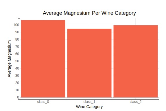
Below We are plotting our first bar chart using bqplot depicting the average magnesium per wine category.
We have first grouped entries of wine dataframe to group entries according to wine categories and then have taken average to collect dataframe with average values of all columns per wine category.
We'll be further using these average values per wine category dataframe in the future with other charts as well.
avg_wine_df = wine_df.groupby(by="Category").mean().reset_index()

avg_wine_df["Category"] = ["class_{}".format(cat) for cat in avg_wine_df.Category]

avg_wine_df
Below, we have created a bar chart using bar() method of pyplot. We have given wine types for x parameter and average magnesium for y parameter.
from bqplot import pyplot as plt

fig = plt.figure(title="Average Magnesium Per Wine Category")

fig.layout.height = "400px"
fig.layout.width = "600px"

bar_chart  = plt.bar(x = avg_wine_df.Category.tolist(), y= avg_wine_df["magnesium"])

bar_chart.colors = ["tomato"]

bar_chart.tooltip = Tooltip(fields=["x", "y"], labels=["Wine Category", "Avg Magnesium"])

plt.xlabel("Wine Category")
plt.ylabel("Average Magnesium")


plt.show()
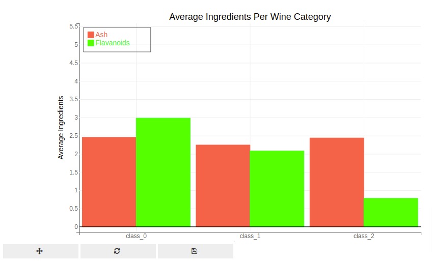
2.2 Grouped Bar Chart 
The below example demonstrates how to generate grouped bar chart using bqplot. We are generating average ash and average flavonoids per wine category as a bar chart.
We have specified chart type by setting type attribute of bar chart object. We can also set chart type using type parameter of bar() method by setting it to setting 'grouped'.
from bqplot import pyplot as plt

fig = plt.figure(title="Average Ingredients Per Wine Category",
                 fig_margin={'top':50, 'bottom':20, 'left':150, 'right':150},
                 legend_location="top-left")

bar_chart  = plt.bar(x = avg_wine_df.Category.tolist(), y= [avg_wine_df["ash"], avg_wine_df["flavanoids"]],
                     labels = ["Ash", "Flavanoids"],
                     display_legend=True)

bar_chart.type = "grouped"

bar_chart.colors = ["tomato", "lime"]

bar_chart.tooltip = Tooltip(fields=["x", "y"], labels=["Wine Category", "Avg Ash/Flavanoids"])

plt.xlabel("Wine Category")
plt.ylabel("Average Ingredients")


plt.show()
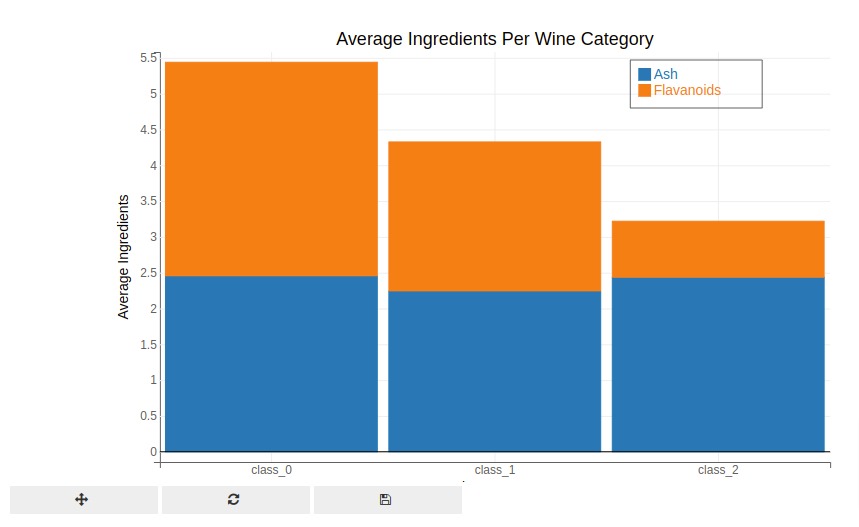
2.3 Stacked bar Chart 
Below we are explaining a stacked bar chart example using bqplot. We are plotting average ash and flavonoids per wine category stacked over one another as a bar chart.
We have created stacked bar chart using exactly same code as that of grouped bar chart with one minor change. We have set type to 'stacked'.
from bqplot import pyplot as plt

fig = plt.figure(title="Average Ingredients Per Wine Category",
                fig_margin={'top':50, 'bottom':20, 'left':150, 'right':150},)

bar_chart  = plt.bar(x = avg_wine_df.Category.tolist(), y= [avg_wine_df["ash"], avg_wine_df["flavanoids"]],
                     labels=["Ash", "Flavanoids"],
                     display_legend=True)

bar_chart.type = "stacked"

bar_chart.colors = bqplot.CATEGORY10

bar_chart.tooltip = Tooltip(fields=["x", "y"], labels=["Wine Category", "Avg Ash/Flavanoids"])

plt.xlabel("Wine Category")
plt.ylabel("Average Ingredients")


plt.show()
3. Line Charts 
The third chart type that we would like to introduce is the famous line chart. We'll be plotting simple line chart as well as chart with more than one line per chart.
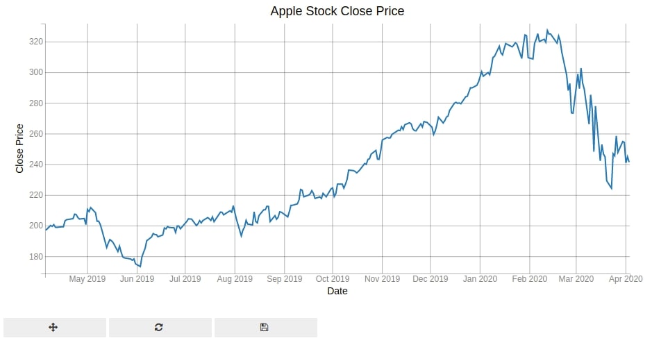
3.1 Apple Stock Close Price Line Chart 
Below we are plotting apple stock close price for the whole period from May 2019 to Apr - 2020. We'll be using plot() method by passing it date-range and closing prices to generate a line chart.
from bqplot import pyplot as plt

fig = plt.figure(title="Apple Stock Close Price")

line_chart = plt.plot(x=apple_df.index, y=apple_df.Close)

plt.xlabel("Date")
plt.ylabel("Close Price")

plt.show()
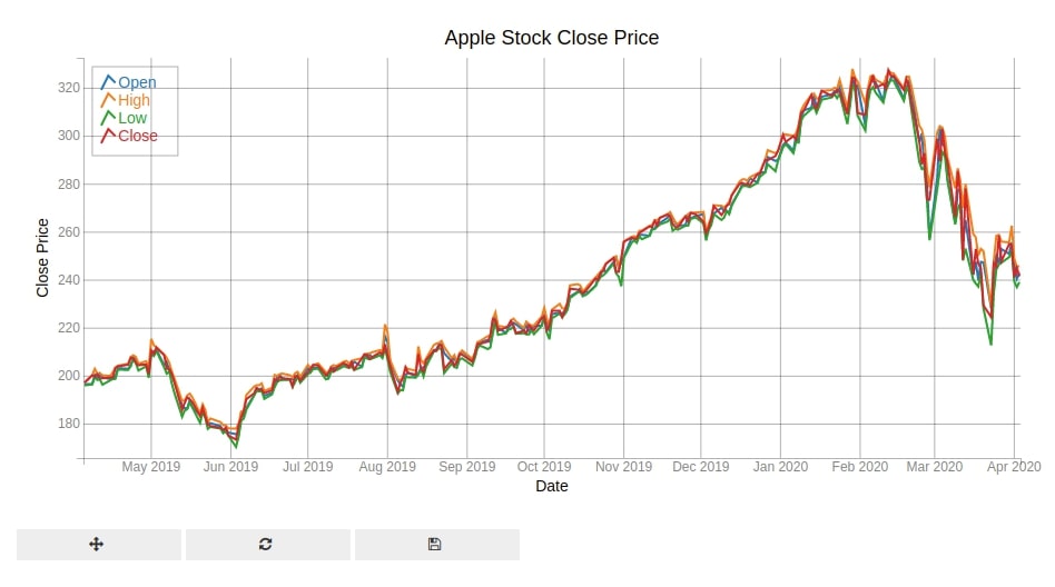
3.2 Apple Stock Open, High, Low and Close Prices Line Charts 
Below we are generating another line chart where we are plotting open, high, low and close prices of apple for a period of May-2019 till Apr-2020. We have combined all line charts in a single figure and also displaying legends to differentiate each line from another using different colors.
from bqplot import pyplot as plt

fig = plt.figure(title="Apple Stock Close Price", legend_location="top-left")

line_chart = plt.plot(x=apple_df.index, y=[apple_df.Open, apple_df.High, apple_df.Low, apple_df.Close],
                     labels=["Open","High", "Low", "Close"],
                     display_legend=True)

plt.xlabel("Date")
plt.ylabel("Close Price")

line_chart.tooltip = Tooltip(fields=["x", "y"], labels=["Date", "OHLC Price"])

plt.show()
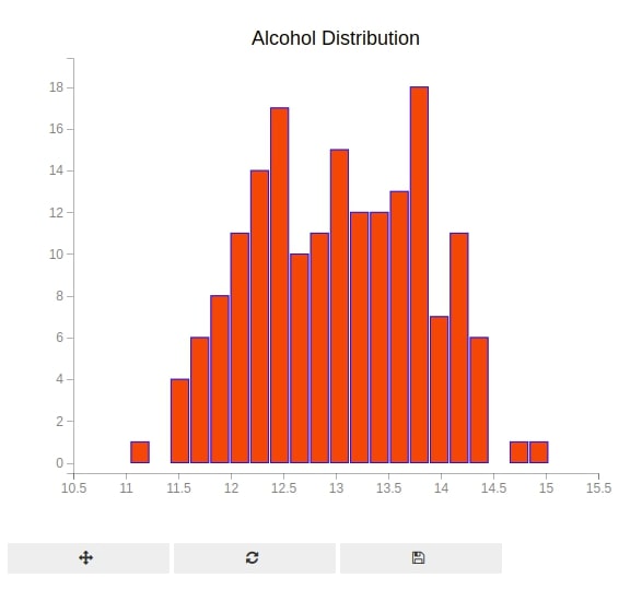
4. Histograms 
The fourth chart type that we'll be introducing is histograms. Histograms are quite commonly used to see a distribution of values of a particular column of data.
Below we are plotting alcohol distribution with 20 bins per histogram. We have created a histogram using hist() method of pyplot.
from bqplot import pyplot as plt

fig = plt.figure(title="Alcohol Distribution")

fig.layout.width = "600px"
fig.layout.height = "500px"

histogram = plt.hist(sample = wine_df["alcohol"], bins=20)

histogram.colors = ["orangered"]
histogram.stroke="blue"
histogram.stroke_width = 2.0

plt.grids(value="none")
plt.xlim(10.5,15.5)

plt.show()
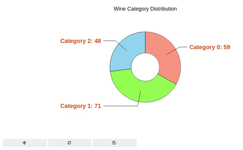
5. Pie Charts (Donut Chart) 
The fifth chart type that we'll introduce is a pie chart.
We have created a pie chart showing distribution of wine categories. We have created a pie chart using pie() method of pyplot. We have calculated wine type count using Counter() functionality available from Python collections module.
Then, we have given counts of wine types to sizes parameter and wine types to labels parameter of pie() method to create a pie chart.
We have also modified various styling attributes of the pie chart.
from collections import Counter

wine_cat = Counter(wine_df["Category"])

wine_cat
from bqplot import pyplot as plt

fig = plt.figure(title="Wine Category Distribution", animation_duration=1000)

pie = plt.pie(sizes = list(wine_cat.values()),
              labels =["Category %d"%val for val in list(wine_cat.keys())],
              display_values = True,
              values_format=".0f",
              display_labels='outside')

pie.stroke="black"
pie.colors = ["tomato","lawngreen", "skyblue"]
pie.opacities = [0.7,0.8,0.9]

pie.radius = 150
pie.inner_radius = 60

pie.label_color = 'orangered'
pie.font_size = '20px'
pie.font_weight = 'bold'

plt.show()
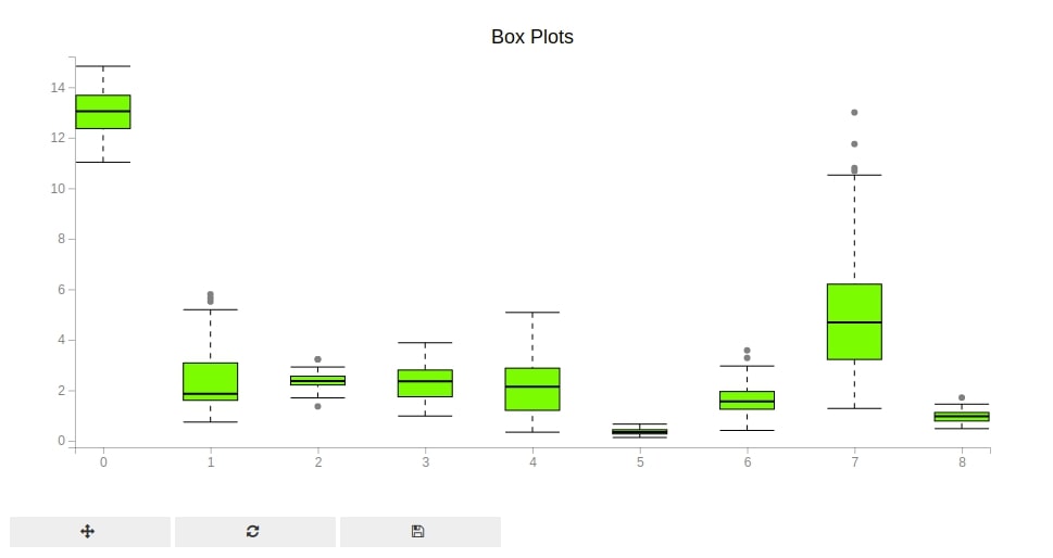
6. Box Plots 
Our sixth chart type is box plots. The box plots are commonly used to check the concentration of the majority of values of a particular quantity. We'll be plotting a box plot for various columns of wine data.
Below, we have created a box plot showing distribution of values of few selected ingredients from wine dataset. We have used boxplot() method of pyplot to create a box plot.
from bqplot import pyplot as plt

fig = plt.figure(title="Box Plots")

mini_df = wine_df[["alcohol","malic_acid","ash","total_phenols", "flavanoids", "nonflavanoid_phenols", "proanthocyanins", "color_intensity", "hue"]]

boxes = plt.boxplot(x=range(mini_df.shape[1]), y=mini_df.values.T)

boxes.box_fill_color = 'lawngreen'
boxes.opacity = 0.6
boxes.box_width = 50

plt.grids(value="none")

plt.show()
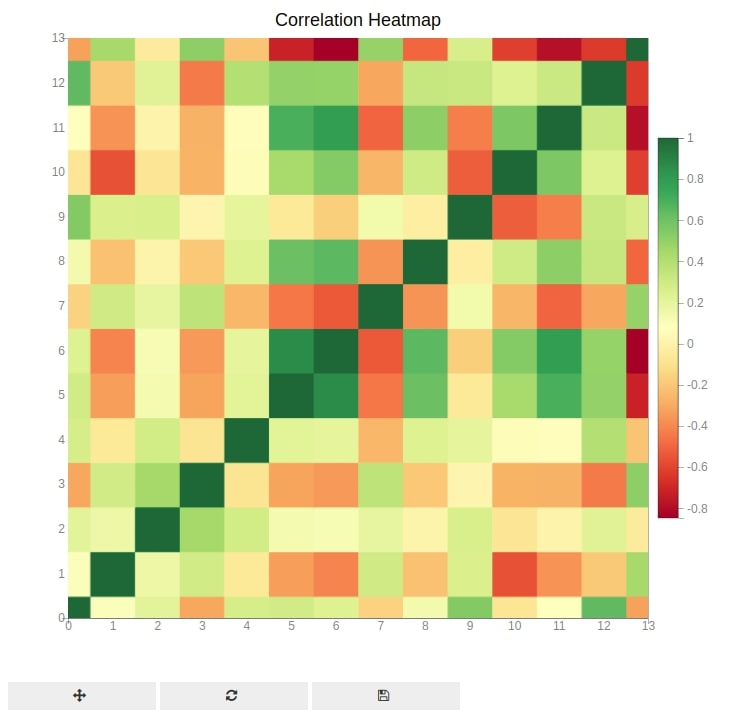
7. HeatMap 
The seventh chart type that we'll be introducing is a heatmap using bqplot. We are using the heatmap below to depict the correlation between various columns of wine data.
First, we have calculated correlation between columns of our wine dataset by calling corr() method on it. Then, we have given that dataframe to color parameter of heatmap() function of pyplot. The heatmap() function is used to create a heatmap using bqplot.
from bqplot import pyplot as plt

fig  = plt.figure(title="Correlation Heatmap",padding_y=0)

fig.layout.width = "700px"
fig.layout.height = "700px"

axes_options = {'color': {'orientation': "vertical","side":"right"}}

plt.heatmap(color=wine_df.corr().values, axes_options=axes_options)

plt.show()
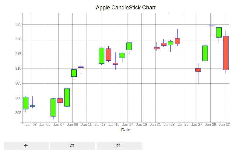
8. Candlestick Charts 
The candlestick charts are very common in the finance industry and our eight chart type that we would like to introduce. It's used to represent a change in the value of the stock for a particular day over a period of time.
8.1 Apple Candlestick Chart with Candle Marker [January - 2020] 
We are plotting a candlestick chart for apple stock for January 2020. We need an open, high, low, and close price of the stock to generate candlestick charts.
We have created a candlestick chart using ohlc() method of pyplot. We have set marker parameter to 'candle' to create a candlestick chart.
from bqplot import pyplot as plt

fig = plt.figure(title="Apple CandleStick Chart")

fig.layout.width="800px"

apple_df_jan_2020 = apple_df["2020-1"]

ohlc = plt.ohlc(x=apple_df_jan_2020.index, y=apple_df_jan_2020[["Open","High","Low","Close"]],
                marker="candle", stroke="blue")

ohlc.colors=["lime", "tomato"]
plt.xlabel("Date")

plt.show()
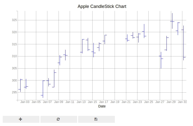
8.2 Apple OHLC Chart [January - 2020] 
Below we have introduced another variation of candlestick chart which only displays lines instead of a bar for each change in stock value.
We have created OHLC chart using ohlc() method of pyplot and setting marker parameter values to 'bar'.
from bqplot import pyplot as plt

fig = plt.figure(title="Apple CandleStick Chart")

fig.layout.width="800px"

apple_df_jan_2020 = apple_df["2020-1"]

ohlc = plt.ohlc(x=apple_df_jan_2020.index, y=apple_df_jan_2020[["Open","High","Low","Close"]],
                marker="bar", stroke="blue")

ohlc.colors=["lime", "tomato"]
plt.xlabel("Date")

plt.show()
9. Choropleth Maps 
Our ninth and last chart type that we'll like to introduce is choropleth maps. bqplot provides a way to create interactive choropleth maps as well. We'll be utilizing the world happiness dataset that we had loaded earlier for plotting various choropleth maps.
We first need to create a simple mapping method that takes as input map data and then maps each id of the country to particular values like happiness score, life expectancy, and corruption of that country. bqplot has a method geo() which is used to generate choropleth mapping needs a mapping from country id to its value to generate choropleth maps as its color parameter.
We'll follow below-mentioned steps to generate choropleth maps with bqplot:
- We'll first generate a world map graph using bqplot's geo(). It'll initialize the graph with data about each country in the world.
- We'll then retrieve map data from bqplot map object and pass it to below function which will generate a mapping from country id to the column.
- We'll then set this mapping from country id to value (like happiness score, life expectancy, corruption perception, etc.) as the color attribute of the map object. We also have set the default color value of grey when we don't find the mapping.
def map_data_to_color_mapping(map_data, column="Score"):
    """
    Function to Map Country ID to Column Value from Happiness DataFrame
    """
    name_to_id_mapping = []
    for entry in map_data:
        if entry["properties"]["name"] == "Russian Federation":
            name_to_id_mapping.append(("Russia", entry["id"]))
        else:
            name_to_id_mapping.append((entry["properties"]["name"], entry["id"]))

    name_to_id_mapping = dict(name_to_id_mapping)

    color = []
    for name, idx in name_to_id_mapping.items():
        score = happiness_df[happiness_df["Country or region"].str.contains(name)]["Score"].values
        if len(score) > 0:
            color.append((idx,score[0]))
    return dict(color)
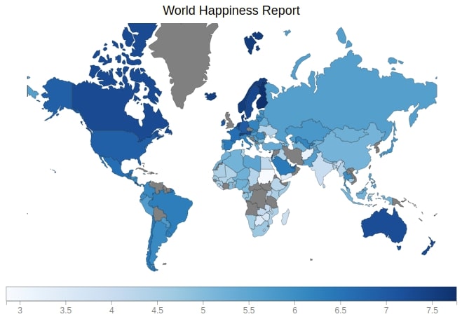
9.1 World Happiness Choropleth Map 
Below we are generating a happiness choropleth map which depicts the choropleth of happiness score for each country of the world.
from bqplot import pyplot as plt

fig = plt.figure(title='World Happiness Report')

plt.scales(scales={'color': bqplot.ColorScale(scheme='Blues')})

choropleth_map = plt.geo(map_data='WorldMap',
                     colors={'default_color': 'Grey'})

map_data = choropleth_map.map_data["objects"]["subunits"]["geometries"]

choropleth_map.color = map_data_to_color_mapping(map_data)

choropleth_map.tooltip = Tooltip(fields=["color"], labels=["Happiness Score"])

fig
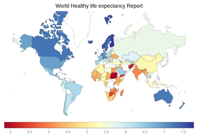
9.2 World Healthy Life Expectancy Choropleth Map 
Below we are generating a Healthy life expectancy choropleth map which depicts choropleth of Healthy life expectancy for each country of the world.
from bqplot import pyplot as plt

fig = plt.figure(title='World Healthy life expectancy Report')

plt.scales(scales={'color': bqplot.ColorScale(scheme='RdYlBu')})

choropleth_map = plt.geo(map_data='WorldMap',
                     colors={'default_color': 'white'})

map_data = choropleth_map.map_data["objects"]["subunits"]["geometries"]

choropleth_map.color = map_data_to_color_mapping(map_data, "Healthy life expectancy")

choropleth_map.tooltip = Tooltip(fields=["color"], labels=["Healthy life expectancy"])

fig
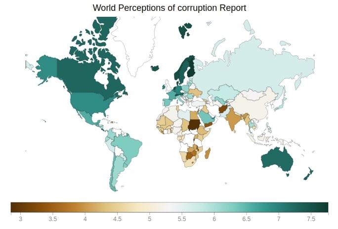
9.3 World Perceptions of Corruption Choropleth Map 
Below we are generating Perceptions of corruption choropleth map which depicts choropleth of Perceptions of corruption for each country of the world.
from bqplot import pyplot as plt

fig = plt.figure(title='World Perceptions of corruption Report')

plt.scales(scales={'color': bqplot.ColorScale(scheme='BrBG')})

choropleth_map = plt.geo(map_data='WorldMap',
                     colors={'default_color': 'white'})

map_data = choropleth_map.map_data["objects"]["subunits"]["geometries"]

choropleth_map.color = map_data_to_color_mapping(map_data, "Perceptions of corruption")

choropleth_map.tooltip = Tooltip(fields=["color"], labels=["Perceptions of corruption"])

fig
This ends our small tutorial on introducing pyplot API of bqplot and various graphs available through this API. Please feel free to let us know your views in the comments section.
References
Other Bqplot Tutorials
- bqplot - Internal Object Model API
- Interactive Maps using bqplot
- Link ipyiwdgets Widgets to Bqplot Charts
- CandleStick Charts using Bqplot
- Bqplot Animation
- bqplot - How to the chart into tooltip of another chart?
Python Data Visualization Libraries
 Sunny Solanki
Sunny Solanki
Intro: Software Developer | Youtuber | Bonsai Enthusiast
About: Sunny Solanki holds a bachelor's degree in Information Technology (2006-2010) from L.D. College of Engineering. Post completion of his graduation, he has 8.5+ years of experience (2011-2019) in the IT Industry (TCS). His IT experience involves working on Python & Java Projects with US/Canada banking clients. Since 2020, he’s primarily concentrating on growing CoderzColumn.
His main areas of interest are AI, Machine Learning, Data Visualization, and Concurrent Programming. He has good hands-on with Python and its ecosystem libraries.
Apart from his tech life, he prefers reading biographies and autobiographies. And yes, he spends his leisure time taking care of his plants and a few pre-Bonsai trees.
Contact: sunny.2309@yahoo.in


![YouTube Subscribe]() Comfortable Learning through Video Tutorials?
Comfortable Learning through Video Tutorials?
If you are more comfortable learning through video tutorials then we would recommend that you subscribe to our YouTube channel.
![Need Help]() Stuck Somewhere? Need Help with Coding? Have Doubts About the Topic/Code?
Stuck Somewhere? Need Help with Coding? Have Doubts About the Topic/Code?
 Stuck Somewhere? Need Help with Coding? Have Doubts About the Topic/Code?
When going through coding examples, it's quite common to have doubts and errors.
If you have doubts about some code examples or are stuck somewhere when trying our code, send us an email at coderzcolumn07@gmail.com. We'll help you or point you in the direction where you can find a solution to your problem.
You can even send us a mail if you are trying something new and need guidance regarding coding. We'll try to respond as soon as possible.
![Share Views]() Want to Share Your Views? Have Any Suggestions?
Want to Share Your Views? Have Any Suggestions?
 Want to Share Your Views? Have Any Suggestions?
If you want to
- provide some suggestions on topic
- share your views
- include some details in tutorial
- suggest some new topics on which we should create tutorials/blogs
 bqplot, interactive-plots