Matplotlib.Pyplot - Complete Guide to Create Charts in Python
Are you looking to create high-quality and publication-ready charts?
Want to create charts using Python?
Which Python data visualization library should you learn first?
Which Python data viz library offers most customization to charts?
If the answer to any of above questions is yes, then you should definitely use Python data visualization library matplotlib.
Matplotlib is the oldest and most stable Python data visualization library that is preferred by developers, data scientists, and ML engineers worldwide to this day.
Many research papers published to this date use matplotlib to create charts.
Now, if you are looking to create charts using Python then matplotlib will be a very good starting point for you. It has a very vast API that let us create many different types of charts and even lets us create animations. Matplotlib charts can be customized a lot compared to other Python data viz libraries.
What Can You Learn From This Article?
As a part of this tutorial, we have explained how to create charts using matplotlib. Tutorial covers a wide variety of chart types like scatter charts, bar charts, line charts, histograms, pie charts, etc. Apart from charts, tutorial also covers how to modify look and feel of charts. Tutorial also covers a guide to using various ready-made themes to improve overall chart aesthetics. If you are someone who is new to matplotlib then this is a good starting point for you.
Below, we have listed important sections of tutorial to give an overview of the material covered.
Important Sections Of Tutorial
- Load Datasets
- Wine Dataset
- Apple OHLC Dataset
- Scatter Plots
- Modify Chart Properties (Axes Labels, Ticks, Title, etc)
- Bar Charts
- Horizontal Bar Chart
- Stacked Bar Chart
- Grouped Bar Chart
- Text Labels Above Bars
- Line Charts
- Step Charts
- Area Charts
- Stacked Area Chart
- Histograms
- Pie Charts
- Donut Chart
- Heatmaps
- Text Labels in Squares
- Box Plots
- Violin Plots
- Hexbin Charts
- Styling Charts (Themes)
Matplotlib Video Tutorial
Please feel free to check below video tutorial if feel comfortable learning through videos. We have covered 6 different chart types in video. But in this tutorial, we have covered many different chart types.
Below, We have imported matplotlib and printed the version that we have used in our tutorial.
import matplotlib

print("Matplotlib Version : {}".format(matplotlib.__version__))
Magic Command to Plot Matplotlib Charts in Jupyter Notebook
In order to display matplotlib charts in Jupyter notebook, we need to call below magic command. Once, we execute below line magic command, we don't need to call show() method as charts will be added to Jupyter notebook.
If you are not aware of what magic commands are then please feel free to check below link. Jupyter notebook let us perform many operations (list directory, load extensions, record execution cell time, etc) in jupyter notebook using magic commands for which otherwise we'll need to use shell or command prompt.
%matplotlib inline
Load Datasets 
In this section, we have loaded datasets that we'll be using to create our charts. We have loaded two datasets for our purpose. Both datasets are loaded as pandas dataframe to make them easily accessible for plotting.
1. Wine Dataset
The first dataset that we'll use for our tutorial is the wine dataset that is available from Python ML library scikit-learn. The dataset has information about various ingredients used in creation of three different types of wines. There is more than one instance of same wine type as ingredients used can be a little different.
from sklearn import datasets
import pandas as pd

wine = datasets.load_wine()

wine_df = pd.DataFrame(wine.data, columns=wine.feature_names)
wine_df["WineType"] = [wine.target_names[wine_typ] for wine_typ in wine.target]

wine_df.head()
2. Apple OHLC Dataset
The second dataset that we'll use for our charting purpose is Apple OHLC dataset which I have downloaded from yahoo finance as a CSV file and loaded in memory as a pandas dataframe. The dataset has apple stock open, close, high, and low prices from Apr 2019 to March 2020.
import pandas as pd

apple_df = pd.read_csv("~/datasets/AAPL.csv", index_col=0, parse_dates=True).reset_index()

apple_df.head()
1. Scatter Plots 
In this section, we have explained how to create scatter charts using matplotlib.
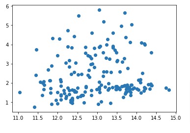
Below, we have created a simple scatter chart showing relationship between alcohol and malic_acid ingredients of wine dataset.
We have created a scatter chart by simply calling scatter() function and giving it a list of values for X and Y axes. For x-axis, we gave a list of alcohol values from wine dataset and for y-axis, we gave a list of malic acid values.
At last, we have called show() function of pyplot to display chart. The call to this method is optional if you are creating charts in Jupyter Notebook and have already called %matplotlib inline command which we executed earlier. Outside of Jupyter notebook, call to this method is required to display charts.
import matplotlib.pyplot as plt

plt.scatter(x=wine_df["alcohol"], y=wine_df["malic_acid"])

plt.show()
Below, we have again created same scatter plot as our previous cell but in a different way. We have given wine dataset to data parameter of scatter() method. Then, we have given X and Y axis simple strings specifying column names from our wine dataset.
The method will take values of those columns from dataset to create scatter chart.
import matplotlib.pyplot as plt

plt.scatter(x="alcohol", y="malic_acid", data=wine_df)

plt.show()
Modify Chart Properties (Axes Labels, Ticks, Title, etc)
In our previous cell, we created a scatter chart with just one line of code but many things were missing over there like there was no axes labels, title, etc. Also, many things were set to default by matplotlib like figure size, point sizes, point color, etc.
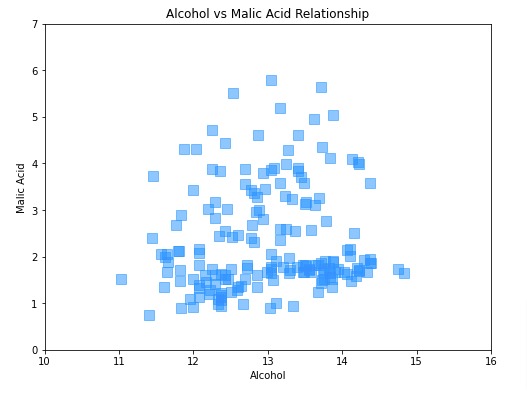
In this section, we have again created a scatter plot showing relationship between alcohol and malic acid but this time we have modified many chart properties to improve the look of the chart.
We have set labels for X and Y axes using xlabel() and ylabel() methods by providing labels as strings to them.
Then, we have set limits for X and Y axis using xlim() and ylim() methods by providing lower and upper bounds.
Then, we have set ticks for X and Y axes using xticks() and yticks() methods. Both methods accept two parameters named ticks and labels. The ticks parameter accepts a list of integers/floats specifying ticks and labels parameter accepts list of values that we need to show for specified ticks. The labels parameter can accepts lists with different types of data like int, float, string, datetime, etc.
We have added a title to chart using title() method which accepts a string as first parameter specifying title of chart.
Apart from these changes, we have modified size of points using s parameter, color using c parameter, marker type using marker parameter, and opacity using alpha parameter of scatter() method.
import matplotlib.pyplot as plt

plt.figure(figsize=(8,6))

plt.scatter(x=wine_df["alcohol"], y=wine_df["malic_acid"],
            s=100, c="dodgerblue", marker="s", alpha=0.5, ## Marker Size, color and opacity.
           )

## Set Axes Labels
plt.xlabel("Alcohol")
plt.ylabel("Malic Acid")

## Set Axes Limits
plt.xlim(10, 16)
plt.ylim(0, 7)

## Set Axes Tick Labels
plt.xticks(ticks=range(10,17), labels=range(10,17))
plt.yticks(ticks=range(8), labels=range(8))

plt.title("Alcohol vs Malic Acid Relationship")

plt.show()
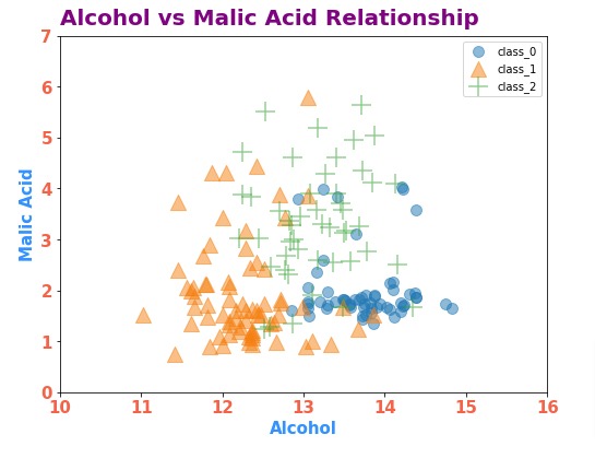
Below, we have created one more example demonstrating how we can modify properties of our scatter chart further. We have again created a scatter chart showing relationship between alcohol and malic acid.
This time, our scatter plot has 3 different types of markers which are based on wine type. We are looping through our three different wine types and creating scatter chart by filtering original dataframe based on selected wine type. We have a dictionary to provide mapping from wine type to color and marker type.
We are calling scatter() method 3 times to create scatter chart for each wine type. We have specified labels for each scatter chart by setting label parameter as wine type.
And we have called legend() method to show legend in chart. It accepts parameter named loc that accepts various string values specifying location of legend. We have set it to 'best' so that it finds best location to put legends that is not overriding chart points. Other useful values for loc parameter are 'upper right', 'upper left', 'lower left', 'lower right', 'right', 'center left', 'center right', 'lower center', 'upper center', and 'center'.
Apart from these changes, we have modified fonts of X-axis, Y-axis, and title. We have specified font properties using fontdict parameter of various methods. The parameter accepts dictionary specifying various font properties like fontsize, fontweight, fontstyle, fontfamily, color, etc.
import matplotlib.pyplot as plt

marker_mapping = {"class_0":"o", "class_1": "^", "class_2":"+"}
size_mapping = {"class_0": 100, "class_1": 200, "class_2": 300}

plt.figure(figsize=(8,6))

for wine_typ in wine_df["WineType"].unique():
    plt.scatter(x=wine_df[wine_df["WineType"]==wine_typ]["alcohol"],
                y=wine_df[wine_df["WineType"]==wine_typ]["malic_acid"],
                marker=marker_mapping[wine_typ], ## Marker Type
                s=size_mapping[wine_typ], ## Marker Size
                alpha=0.5, ## Marker opacity.
                label=wine_typ
               )

## Set Axes Labels
plt.xlabel("Alcohol", fontdict=dict(fontsize=15, fontweight="bold", color="dodgerblue"))
plt.ylabel("Malic Acid", fontdict=dict(fontsize=15, fontweight="bold", color="dodgerblue"))

## Set Axes Limits
plt.xlim(10, 16)
plt.ylim(0, 7)

## Set Axes Tick Labels
plt.xticks(ticks=range(10,17), labels=range(10,17), fontdict=dict(fontsize=15, fontweight="bold", color="tomato"))
plt.yticks(ticks=range(8), labels=range(8), fontdict=dict(fontsize=15, fontweight="bold", color="tomato"))

plt.title("Alcohol vs Malic Acid Relationship", loc="left",
          fontdict=dict(fontsize=20, fontweight="bold", color="purple"), pad=10)

plt.legend(loc="best")

plt.show()
2. Bar Charts 
In this section, we'll explain how to create bar charts and their different versions (stacked, grouped, etc) using matplotlib.
Below, we have first created a new dataframe that we'll be using for creating bar charts. The dataframe is created by grouping entries of original wine dataframe based on wine type and then taking mean of values. The final dataframe has average values of ingredients per wine type.
avg_wine_df = wine_df.groupby("WineType").mean().reset_index()

avg_wine_df
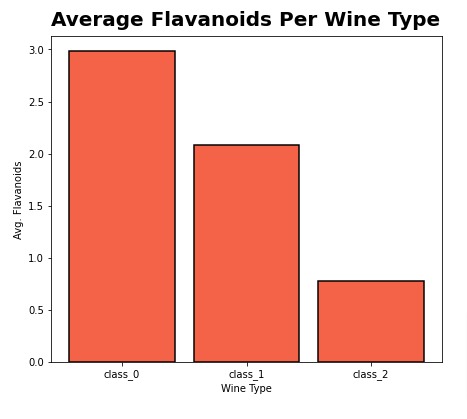
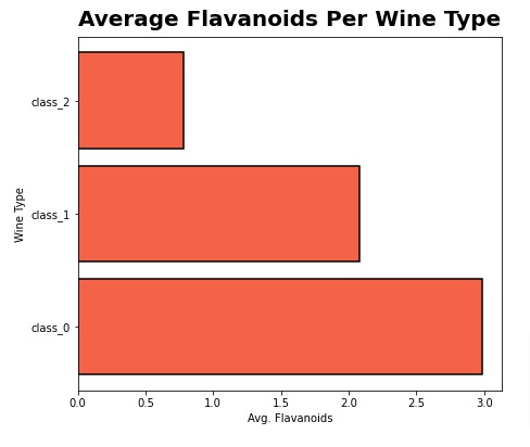
Below, we have created a bar chart showing average flavanoids used per wine type. We have created bar chart by calling bar() function of pyplot. For x-axis values, we have provided list of wine types and for height of bars, we have provided average flavanoids values from dataframe.
We can provide bar width using width parameter. It accepts float in the range of 0-1. The default value is 0.8.
We can also modify edge width and color of line around bars using edgecolor and linewidth parameters.
import matplotlib.pyplot as plt

plt.figure(figsize=(7,6))

plt.bar(x=avg_wine_df["WineType"], height=avg_wine_df["flavanoids"],
        width=0.85, color="tomato", edgecolor="black", linewidth=1.5
       )

## Set Axes Labels
plt.xlabel("Wine Type")
plt.ylabel("Avg. Flavanoids")

plt.title("Average Flavanoids Per Wine Type", loc="left", fontdict=dict(fontsize=20, fontweight="bold"), pad=10)

plt.show()
2.1 Horizontal Bar Chart
In this section, we have explained how to create horizontal bar chart using matplotlib. We have again created bar chart showing average flavanoids used per wine type.
In order to create horizontal bar chart, we have used barh() function of pyplot instead. We have provided wine types to Y-axis and average flavanoids values as bar widths. All bar's height is set to fix value.
import matplotlib.pyplot as plt

plt.figure(figsize=(7,6))

plt.barh(y=avg_wine_df["WineType"], width=avg_wine_df["flavanoids"],
         height=0.85, color="tomato",
         edgecolor="black", linewidth=1.5
       )

## Set Axes Labels
plt.xlabel("Avg. Flavanoids")
plt.ylabel("Wine Type")

plt.title("Average Flavanoids Per Wine Type", loc="left", fontdict=dict(fontsize=20, fontweight="bold"), pad=10)

plt.show()
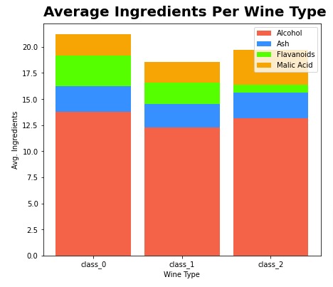
2.2 Stacked Bar Chart
In this section, we'll explain how to create stacked bar chart using matplotlib. We'll be creating stacked bar chart showing average values of 4 ingredients (alcohol, ash, flavanoids, and malic acid) per wine type.
In order to create stacked bar chart, we have again used bar() function from pyplot. The only difference this time is that we have used bottom parameter of function to specify from where bar should start.
For first alcohol bars, we don't need to specify bottom because it starts at 0. For second ash values bars, we need to specify bottom values as alcohol values because we want to start ash after alcohol. For third flavanoids, we need to specify bottom values as sum of alcohol and ash values. For malic acid, we need to specify bottom values as sum of alcohol, ash, and flavanoids values. This way bars will be stacked one over another.
Apart from bottom, we have set different colors for bars based on ingredient name and also set label as ingredient name to show them in legend.
import matplotlib.pyplot as plt

plt.figure(figsize=(7,6))

plt.bar(x=avg_wine_df["WineType"], height=avg_wine_df["alcohol"], width=0.85, color="tomato", label="Alcohol")
plt.bar(x=avg_wine_df["WineType"], height=avg_wine_df["ash"],
        bottom=avg_wine_df["alcohol"], width=0.85, color="dodgerblue", label="Ash")
plt.bar(x=avg_wine_df["WineType"], height=avg_wine_df["flavanoids"],
        bottom=avg_wine_df[["ash", "alcohol"]].sum(axis=1), width=0.85, color="lime", label="Flavanoids")
plt.bar(x=avg_wine_df["WineType"], height=avg_wine_df["malic_acid"],
        bottom=avg_wine_df[["alcohol", "ash", "flavanoids"]].sum(axis=1), width=0.85, color="orange", label="Malic Acid")


## Set Axes Labels
plt.xlabel("Wine Type")
plt.ylabel("Avg. Ingredients")

plt.title("Average Ingredients Per Wine Type", loc="left", fontdict=dict(fontsize=20, fontweight="bold"), pad=10)

plt.legend(loc='best')

plt.show()
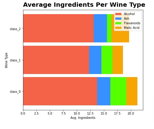
Below, we have created one more example of stacked bar chart but we have laid bars horizontally instead of vertically (horizontal stacked bar chart).
We have created horizontal stacked bar chart using barh() function of pyplot.
import matplotlib.pyplot as plt

plt.figure(figsize=(7,6))

plt.barh(y=avg_wine_df["WineType"], width=avg_wine_df["alcohol"], height=0.9, color="tomato", label="Alcohol")
plt.barh(y=avg_wine_df["WineType"], width=avg_wine_df["ash"],
        left=avg_wine_df["alcohol"], height=0.9, color="dodgerblue", label="Ash")
plt.barh(y=avg_wine_df["WineType"], width=avg_wine_df["flavanoids"],
        left=avg_wine_df[["ash", "alcohol"]].sum(axis=1), height=0.9, color="lime", label="Flavanoids")
plt.barh(y=avg_wine_df["WineType"], width=avg_wine_df["malic_acid"],
        left=avg_wine_df[["alcohol", "ash", "flavanoids"]].sum(axis=1), height=0.9, color="orange", label="Malic Acid")


## Set Axes Labels
plt.xlabel("Avg. Ingredients")
plt.ylabel("Wine Type")

plt.title("Average Ingredients Per Wine Type", loc="left", fontdict=dict(fontsize=20, fontweight="bold"), pad=10)

plt.legend(loc='best')

plt.show()
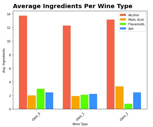
2.3 Grouped Bar Chart
In this section, we'll explain how to create grouped bar chart using matplotlib. We'll be creating grouped bar chart showing average values of 4 ingredients (alcohol, malic acid, flavanoids, and ash) per wine type.
Below, we have created grouped bar chart by calling bar() function for each ingredient. The only difference this time is that we have used custom values for x axis to set bars next to each other.
We have also set custom values for x axis ticks. The rest of the code is almost same as in our previous examples.
import matplotlib.pyplot as plt

plt.figure(figsize=(8,6))

plt.bar(x=[0,5,10], height=avg_wine_df["alcohol"], width=0.9, color="tomato", label="Alcohol")
plt.bar(x=[1,6,11], height=avg_wine_df["malic_acid"], width=0.9, color="orange", label="Malic Acid")
plt.bar(x=[2,7,12], height=avg_wine_df["flavanoids"], width=0.9, color="lime", label="Flavanoids")
plt.bar(x=[3,8,13], height=avg_wine_df["ash"], width=0.9, color="dodgerblue", label="Ash")

## Set Axes Labels
plt.xlabel("Wine Type")
plt.ylabel("Avg. Ingredients")

plt.xticks(ticks=[1.5, 6.5, 11.5], labels=avg_wine_df["WineType"], rotation=45)

plt.title("Average Ingredients Per Wine Type", loc="left", fontdict=dict(fontsize=20, fontweight="bold"), pad=10)

plt.legend(loc='best')

plt.show()
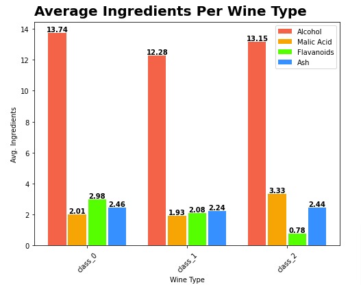
Below, we have recreated our grouped bar chart from previous cell but this time we have added text labels specifying average ingredient value above each bar.
We have introduced text labels by calling text() function from pyplot. It accepts (x,y) coordinates of text and text itself to add text labels at specified coordinates. The ha and va parameters are used to specify horizontal and vertical alignment. The ha parameter accepts values like 'center', 'left' and 'right' whereas va parameter accepts values like 'top', 'bottom' and 'center'.
import matplotlib.pyplot as plt

plt.figure(figsize=(8,6))

plt.bar(x=[0,5,10], height=avg_wine_df["alcohol"], width=0.9, color="tomato", label="Alcohol")
plt.bar(x=[1,6,11], height=avg_wine_df["malic_acid"], width=0.9, color="orange", label="Malic Acid")
plt.bar(x=[2,7,12], height=avg_wine_df["flavanoids"], width=0.9, color="lime", label="Flavanoids")
plt.bar(x=[3,8,13], height=avg_wine_df["ash"], width=0.9, color="dodgerblue", label="Ash")

## Add Text Above Bars
for x, y in zip([0,1,2,3,5,6,7,8,10,11,12,13], avg_wine_df[["alcohol", "malic_acid", "flavanoids", "ash"]].values.flatten()):
    plt.text(x, y, "{:.2f}".format(y), ha="center", va="bottom", fontdict=dict(fontsize=10, fontweight="bold"))

## Set Axes Labels
plt.xlabel("Wine Type")
plt.ylabel("Avg. Ingredients")

## Set Tick Labels
plt.xticks(ticks=[1.5, 6.5, 11.5], labels=avg_wine_df["WineType"], rotation=45)

plt.title("Average Ingredients Per Wine Type", loc="left", fontdict=dict(fontsize=20, fontweight="bold"), pad=10)

plt.legend(loc='best')

plt.show()
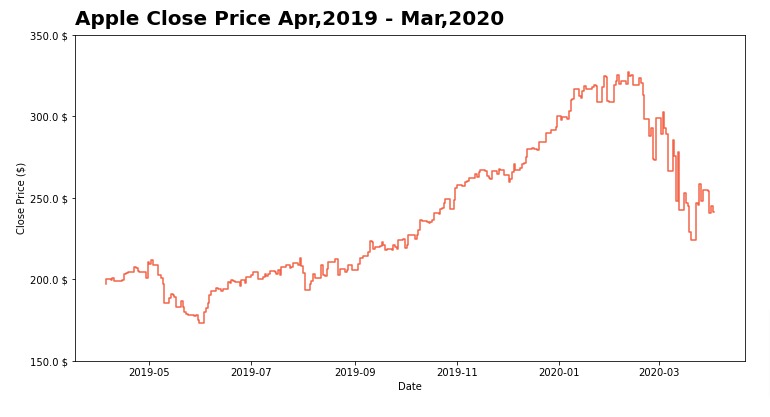
3. Line Charts 
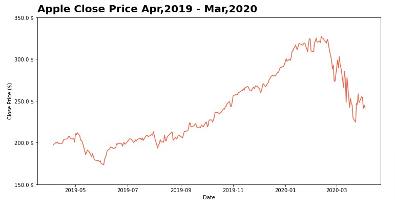
In this section, we have explained how to create line chart using matplotlib. We have created line chart showing close prices of apple stock over time.
We have created line chart by calling plot() function of pyplot module. We have provided date values from apple dataframe for x-axis and close prices for y-axis.
import matplotlib.pyplot as plt

plt.figure(figsize=(12,6))

plt.plot(apple_df["Date"], apple_df["Close"], color="tomato")

## Set Axes Labels
plt.xlabel("Date")
plt.ylabel("Close Price ($)")

## Set Tick Labels
plt.yticks(ticks=range(150,400,50), labels=map(lambda x: "{:.1f} $".format(x), range(150,400,50)))

plt.title("Apple Close Price Apr,2019 - Mar,2020", loc="left", fontdict=dict(fontsize=20, fontweight="bold"), pad=10)

plt.show()
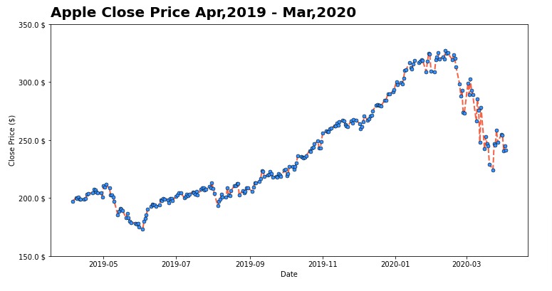
Below, we have again created a line chart but this time, we have used different markers by setting marker parameter to introduce circles in chart. The marker parameter accepts values like 'o', '^', 's', '+'* and many more.
We have also set markersize, markerfacecolor, markeredgecolor, and markeredgewidth parameters.
We can specify line style using linestyle parameter. It accepts values like 'dashed', 'dotted', '-.', '--' and many more.
import matplotlib.pyplot as plt

plt.figure(figsize=(12,6))

plt.plot(apple_df["Date"], apple_df["Close"], color="tomato",
         linewidth=2.0, linestyle="dashed", ## Line Attribtues
         marker="o", markersize=5, markerfacecolor="dodgerblue", markeredgecolor="black", markeredgewidth=0.5 ## Marker Attributes
        )

## Set Axes Labels
plt.xlabel("Date")
plt.ylabel("Close Price ($)")

## Set Tick Labels
plt.yticks(ticks=range(150,400,50), labels=map(lambda x: "{:.1f} $".format(x), range(150,400,50)))

plt.title("Apple Close Price Apr,2019 - Mar,2020", loc="left", fontdict=dict(fontsize=20, fontweight="bold"), pad=10)

plt.show()
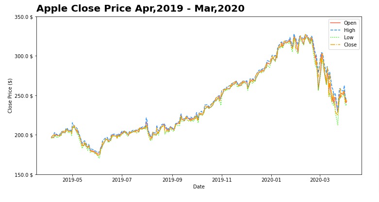
Below, we have created one more example explaining how to create line chart using matplotlib. This time we have created a line chart with 4 lines. We have plotted all 4 prices (open, high, low, and close) of apple stock on chart. We have used different line styles and colors to separate them from each other.
import matplotlib.pyplot as plt

plt.figure(figsize=(12,6))

plt.plot(apple_df["Date"], apple_df["Open"], color="tomato", label="Open")
plt.plot(apple_df["Date"], apple_df["High"], color="dodgerblue", linestyle="dashed", label="High")
plt.plot(apple_df["Date"], apple_df["Low"], color="lime", linestyle="dotted", label="Low")
plt.plot(apple_df["Date"], apple_df["Close"], color="orange", linestyle="-.", label="Close")

## Set Axes Labels
plt.xlabel("Date")
plt.ylabel("Close Price ($)")

### Set X ticks
plt.yticks(ticks=range(150,400,50), labels=map(lambda x: "{:.1f} $".format(x), range(150,400,50)))

plt.title("Apple Close Price Apr,2019 - Mar,2020", loc="left", fontdict=dict(fontsize=20, fontweight="bold"), pad=10)

plt.legend(loc="best")

plt.show()
4. Step Charts 
In this section, we'll explain how to create step charts using matplotlib. The step chart is another type of line chart only. We have created a simple step chart showing close price of apple stock over time.
We have created step chart using step() function of pyplot. The rest of the code is same as line chart.
import matplotlib.pyplot as plt

plt.figure(figsize=(12,6))

plt.step(apple_df["Date"], apple_df["Close"], color="tomato")

## Set Axes Labels
plt.xlabel("Date")
plt.ylabel("Close Price ($)")

## Set Tick Labels
plt.yticks(ticks=range(150,400,50), labels=map(lambda x: "{:.1f} $".format(x), range(150,400,50)))

plt.title("Apple Close Price Apr,2019 - Mar,2020", loc="left", fontdict=dict(fontsize=20, fontweight="bold"), pad=10)

plt.show()
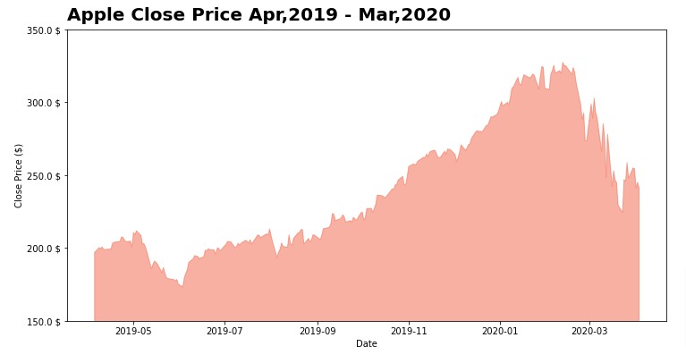
5. Area Charts 
In this section, we'll explain how to create area charts using matplotlib. We have created an area chart covering area below close price of apple stock over time.
We have created an area chart using fill_between() function available from pyplot module. The function accepts three parameters which are x, y1, and y2. It'll fill an area between y1 and y2. We can provide single value or list of values to these parameters.
In our case, we have used date values for x-axis and close prices for y1. The y2 will be set to 0 by default and ignored. This will fill area below y1 which is close prices in our case.
import matplotlib.pyplot as plt

plt.figure(figsize=(12,6))

plt.fill_between(x=apple_df["Date"], y1=apple_df["Close"], color="tomato", alpha=0.5)

## Set Axes Labels
plt.xlabel("Date")
plt.ylabel("Close Price ($)")

plt.ylim(150,350)

## Set Tick Labels
plt.yticks(ticks=range(150,400,50), labels=map(lambda x: "{:.1f} $".format(x), range(150,400,50)))

plt.title("Apple Close Price Apr,2019 - Mar,2020", loc="left", fontdict=dict(fontsize=20, fontweight="bold"), pad=10)

plt.show()
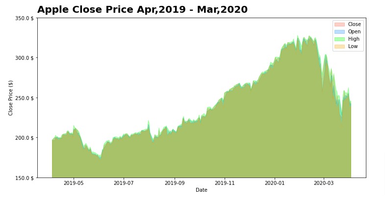
Below, we have created another example of area chart where we have covered area of more than one data variable. We have covered area below all 4 prices of apple stock.
import matplotlib.pyplot as plt

plt.figure(figsize=(12,6))

plt.fill_between(x=apple_df["Date"], y1=apple_df["Close"], color="tomato", alpha=0.3, label="Close")
plt.fill_between(x=apple_df["Date"], y1=apple_df["Open"], color="dodgerblue", alpha=0.3, label="Open")
plt.fill_between(x=apple_df["Date"], y1=apple_df["High"], color="lime", alpha=0.3, label="High")
plt.fill_between(x=apple_df["Date"], y1=apple_df["Low"], color="orange", alpha=0.3, label="Low")

## Set Axes Labels
plt.xlabel("Date")
plt.ylabel("Close Price ($)")

plt.ylim(150,350)

## Set Tick Labels
plt.yticks(ticks=range(150,400,50), labels=map(lambda x: "{:.1f} $".format(x), range(150,400,50)))

plt.title("Apple Close Price Apr,2019 - Mar,2020", loc="left", fontdict=dict(fontsize=20, fontweight="bold"), pad=10)

plt.legend(loc="best")

plt.show()
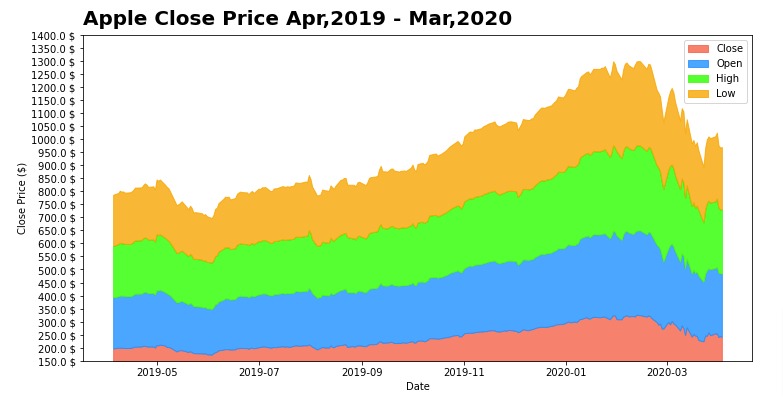
5.1 Stacked Area Chart
In this section, we have explained how to create a stacked area chart using matplotlib. We have again used fill_between() function to create area chart. We have stacked area of open, high, low, and close prices on one another.
In order to create a stacked bar chart, we have provided y2 parameter values this time. For close price, y2 is not specified as it is first lower area chart. For open values area chart, y1 is set as close prices, and y2 is set as sum of open and close prices. The same logic is followed for other stacked areas as well.
import matplotlib.pyplot as plt

plt.figure(figsize=(12,6))

plt.fill_between(x=apple_df["Date"], y1=apple_df["Close"], color="tomato", alpha=0.8, label="Close")
plt.fill_between(x=apple_df["Date"], y1=apple_df["Close"], y2=apple_df[["Open", "Close"]].sum(axis=1),
                 color="dodgerblue", alpha=0.8, label="Open")
plt.fill_between(x=apple_df["Date"], y1=apple_df[["Open", "Close"]].sum(axis=1),
                 y2=apple_df[["Open", "Close", "High"]].sum(axis=1),
                 color="lime", alpha=0.8, label="High")
plt.fill_between(x=apple_df["Date"], y1=apple_df[["Open", "Close", "High"]].sum(axis=1),
                 y2=apple_df[["Open", "Close", "High", "Low"]].sum(axis=1),
                 color="orange", alpha=0.8, label="Low")

## Set Axes Labels
plt.xlabel("Date")
plt.ylabel("Close Price ($)")

plt.ylim(150,1400)

## Set Tick Labels
plt.yticks(ticks=range(150,1450,50), labels=map(lambda x: "{:.1f} $".format(x), range(150,1450,50)))

plt.title("Apple Close Price Apr,2019 - Mar,2020", loc="left", fontdict=dict(fontsize=20, fontweight="bold"), pad=10)

plt.legend(loc="best")

plt.show()
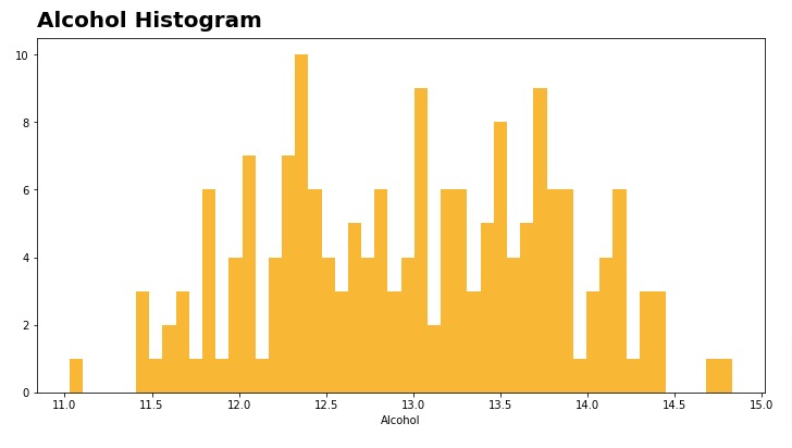
6. Histograms 
In this section, we have explained how to create histograms using matplotlib. We have created a simple histogram of alcohol values from our wine dataset.
We can create histogram using hist() function available from pyplot module. We have provided list of alcohol values for creating histogram. We can specify bin size using bins parameter of function.
import matplotlib.pyplot as plt

plt.figure(figsize=(12,6))

plt.hist(x=wine_df["alcohol"], bins=50, color="orange", alpha=0.8)

## Set Axes Labels
plt.xlabel("Alcohol")

plt.title("Alcohol Histogram", loc="left", fontdict=dict(fontsize=20, fontweight="bold"), pad=10)

plt.show()
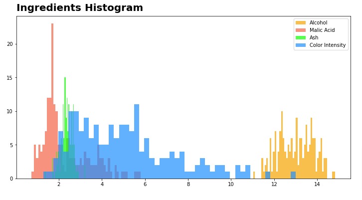
Below, we have created one more example demonstrating histogram creation using matplotlib. This time, we have created histogram of 4 different ingredients (alcohol, malic acid, ash, and color intensity) from our wine dataset.
import matplotlib.pyplot as plt

plt.figure(figsize=(12,6))

plt.hist(x=wine_df["alcohol"], bins=50, color="orange", alpha=0.7, label="Alcohol")
plt.hist(x=wine_df["malic_acid"], bins=50, color="tomato", alpha=0.7, label="Malic Acid")
plt.hist(x=wine_df["ash"], bins=50, color="lime", alpha=0.7, label="Ash")
plt.hist(x=wine_df["color_intensity"], bins=50, color="dodgerblue", alpha=0.7, label="Color Intensity")

plt.title("Ingredients Histogram", loc="left", fontdict=dict(fontsize=20, fontweight="bold"), pad=10)

plt.legend(loc="best")

plt.show()
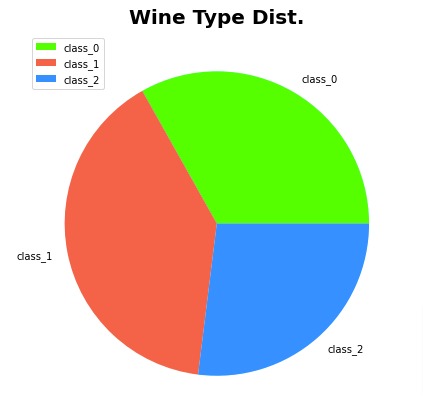
7. Pie Charts 
In this section, we have explained how to create pie charts using matplotlib. We have created pie chart showing distribution of data examples based on wine type from our wine dataset.
Below, we have created new dataframe that has information about data examples count based on wine type. We'll use it to create pie chart.
wine_df_cnt = wine_df.groupby("WineType").count()[["alcohol"]].rename(columns={"alcohol":"Count"}).reset_index()

wine_df_cnt
Below, we have created pie chart showing distribution of data examples based on wine type using pie() function. The first parameter x is provided with list of counts of data examples. The labels parameter accepts list specifying labels for wedges. The colors parameter accepts list of colors for wedges.
import matplotlib.pyplot as plt

plt.figure(figsize=(7,7))

plt.pie(x=wine_df_cnt["Count"], labels=wine_df_cnt["WineType"], colors=["lime", "tomato", "dodgerblue"])

plt.title("Wine Type Dist.", fontdict=dict(fontsize=20, fontweight="bold"), pad=10)

plt.legend(loc="best")

plt.show()
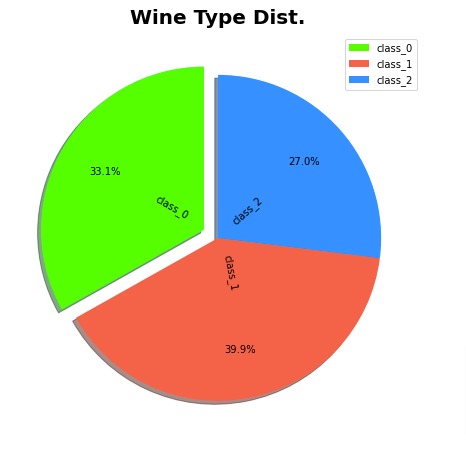
Below, we have again created same pie chart as our previous cell showing distribution of data examples based on wine type. We have modified few chart properties this time.
We have informed chart to take wedge of class_0 little out to draw attention to it using explode parameter. It accepts list of floats in the range of 0-1. The list has same length as number of wedges. As we wanted the wedge of class_0 to be little out, we have set its value to 0.1 and 0.0 for all others.
The autopct parameter let us specify format of percentage displayed. The pctdistance parameter let us specify distance of percentage labels from center.
We can also inform chart to start wedges from different angle using startangle parameter.
The labeldistance parameter is used to specify distance of label from center. The rotatelabels parameter accepts boolean value specifying whether to rotate labels or not. The shadow parameter simply adds shadow to wedges.
import matplotlib.pyplot as plt

plt.figure(figsize=(7.5,7.5))

plt.pie(x=wine_df_cnt["Count"], labels=wine_df_cnt["WineType"],
        explode=[0.1,0.,0.], shadow=True, labeldistance=0.1,
        autopct='%1.1f%%', pctdistance=0.7, startangle=90, rotatelabels=True,
        colors=["lime", "tomato", "dodgerblue"])

plt.title("Wine Type Dist.", fontdict=dict(fontsize=20, fontweight="bold"), pad=10)

plt.legend(loc="best")

plt.show()
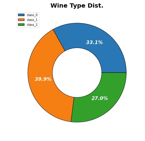
7.1 Donut Chart
In this example, we have explained how to create donut chart using matplotlib. We can create donut chart using our same pie() function.
In order to create donut chart, we need to use wedgeprops parameter of function. We can specify width of wedge over there. We can also modify other things like wedge edge color, width, etc.
Apart from this, we have also modified chart text labels using textprops parameter.
import matplotlib.pyplot as plt

plt.figure(figsize=(7.5,7.5))

plt.pie(x=wine_df_cnt["Count"], labels=wine_df_cnt["WineType"],
        autopct='%1.1f%%', pctdistance=0.7,
        wedgeprops=dict(width=0.5, edgecolor="black"),
        textprops=dict(color="w", fontsize=16, fontstyle="italic", fontweight="bold")
       )

plt.title("Wine Type Dist.", fontdict=dict(fontsize=20, fontweight="bold"), pad=10)

plt.legend(loc="best")

plt.show()
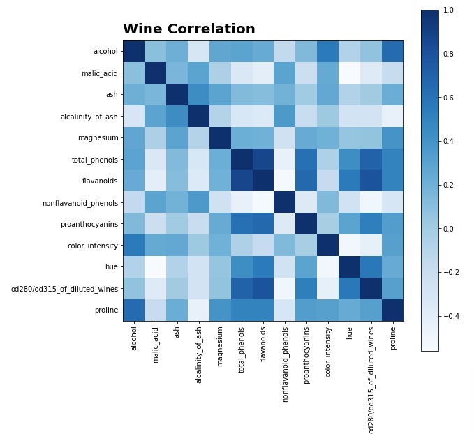
8. Heatmaps 
In this section, we have explained how to create heatmaps using matplotlib. We have created a heatmap showing correlation between ingredients of our wine dataset.
Below, we have first calculated correlation using corr() function of pandas. We'll be using this new dataframe to create heatmap.
wine_corr_df = wine_df.corr()

wine_corr_df
Below, we have created heatmap using imshow() function of pyplot module. We have provided our correlation dataframe to function. We have also specified color map using cmap parameter.
Apart from this, we have also added color bar to chart by calling colorbar() function of pyplot.
import matplotlib.pyplot as plt

plt.figure(figsize=(9,9))

plt.imshow(wine_corr_df, cmap="Blues")

plt.colorbar()

## Set tick labels
plt.xticks(range(13), wine_corr_df.index, rotation=90)
plt.yticks(range(13), wine_corr_df.index)

plt.title("Wine Correlation", loc="left", fontdict=dict(fontsize=20, fontweight="bold"), pad=10)

plt.show()
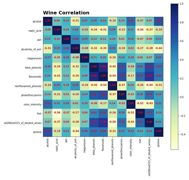
Below, we have created one more example of creating heatmap. We have again created same heatmap as previous cell showing correlation between ingredients of wine dataset but this time, we have added correlation values as text in each square. This gives us more details compared to our previous chart.
import matplotlib.pyplot as plt

plt.figure(figsize=(11,11))

plt.imshow(wine_corr_df, cmap="YlGnBu")

plt.colorbar(location="right")

## Set tick labels
plt.xticks(range(13), wine_corr_df.index, rotation=90)
plt.yticks(range(13), wine_corr_df.index)

## Add Correlation texts
for i in range(13):
    for j in range(13):
        plt.text(i,j, "{:.2f}".format(wine_corr_df.values[i,j]), ha="center", color="red", fontweight="bold")

plt.title("Wine Correlation", loc="left", fontdict=dict(fontsize=20, fontweight="bold"), pad=10)

plt.show()
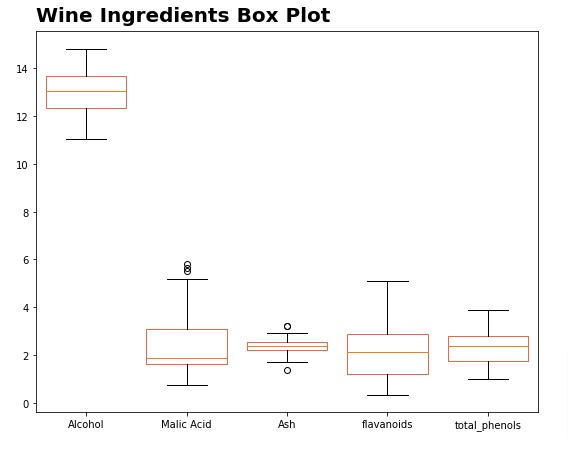
9. Box Plots 
In this section, we have explained how to create box plots using matplotlib. We have created box plot for few selected ingredients of our wine dataset.
We can create box plot using boxplot() function of pyplot module. We have provided it list of ingredient values to create box plot.
import matplotlib.pyplot as plt

plt.figure(figsize=(9,7))

plt.boxplot(x=[wine_df["alcohol"], wine_df["malic_acid"], wine_df["ash"], wine_df["flavanoids"], wine_df["total_phenols"]],
            labels=["Alcohol", "Malic Acid", "Ash", "flavanoids", "total_phenols"],
            widths=0.8,
            boxprops=dict(color="tomato"),
           )

plt.title("Wine Ingredients Box Plot", loc="left", fontdict=dict(fontsize=20, fontweight="bold"), pad=10)

plt.show()
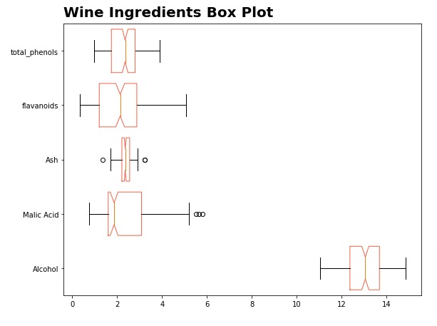
Below, we have created one more example demonstrating creation of box plot. This time, we have created a horizontal box plot with same ingredients as our previous chart. We can create horizontal box plot by setting vert parameter to False.
import matplotlib.pyplot as plt

plt.figure(figsize=(9,7))

plt.boxplot(x=[wine_df["alcohol"], wine_df["malic_acid"], wine_df["ash"], wine_df["flavanoids"], wine_df["total_phenols"]],
            labels=["Alcohol", "Malic Acid", "Ash", "flavanoids", "total_phenols"],
            widths=0.8, vert=False, notch=True,
            boxprops=dict(color="tomato"),
           )

plt.title("Wine Ingredients Box Plot", loc="left", fontdict=dict(fontsize=20, fontweight="bold"), pad=10)

plt.show()
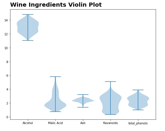
10. Violin Plots 
In this section, we have explained how to create violin plot using matplotlib. We have created violin plot showing distribution of values for selected ingredients from our wine dataset.
We have created violin plot using violinplot() function available from pyplot module.
import matplotlib.pyplot as plt

plt.figure(figsize=(9,7))

plt.violinplot([wine_df["alcohol"], wine_df["malic_acid"], wine_df["ash"], wine_df["flavanoids"], wine_df["total_phenols"]],
               widths=0.8)

plt.xticks(range(1, 6),["Alcohol", "Malic Acid", "Ash", "flavanoids", "total_phenols"])

plt.title("Wine Ingredients Violin Plot", loc="left", fontdict=dict(fontsize=20, fontweight="bold"), pad=10)

plt.show()
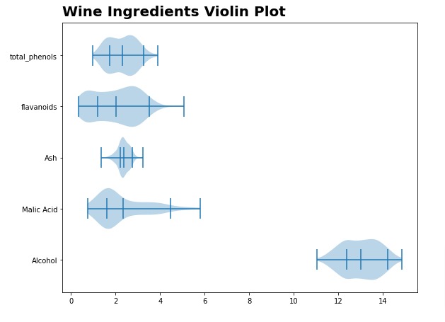
Below, we have created one more example showing how to create violin plot. This time, we have created horizontal violin plot. We can set it to horizontal by setting vert parameter to False.
import matplotlib.pyplot as plt

plt.figure(figsize=(9,7))

plt.violinplot([wine_df["alcohol"], wine_df["malic_acid"], wine_df["ash"], wine_df["flavanoids"], wine_df["total_phenols"]],
               widths=0.8, vert=False, showmeans=True, quantiles=[(0.25, 0.95),] *5)

plt.yticks(range(1, 6),["Alcohol", "Malic Acid", "Ash", "flavanoids", "total_phenols"])

plt.title("Wine Ingredients Violin Plot", loc="left", fontdict=dict(fontsize=20, fontweight="bold"), pad=10)

plt.show()
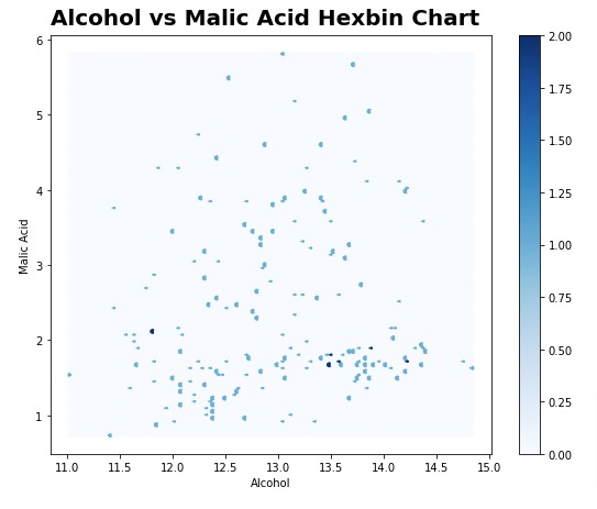
11. Hexbin 
In this section, we have explained how to create hebin chart using matplotlib. We have created hexbin chart showing relationship between alcohol and malic acid ingredients of wine dataset. The chart highlights number of examples where values match.
We can create a hexbin chart using hexbin() function of pyplot module. We have provided alcohol and malic acid values to it. We have specified color map using cmap parameter.
import matplotlib.pyplot as plt

plt.figure(figsize=(9,7))

plt.hexbin(wine_df["alcohol"], wine_df["malic_acid"], cmap="Blues")

plt.colorbar()

plt.xlabel("Alcohol")
plt.ylabel("Malic Acid")

plt.title("Alcohol vs Malic Acid Hexbin Chart", loc="left", fontdict=dict(fontsize=20, fontweight="bold"), pad=10)

plt.show()
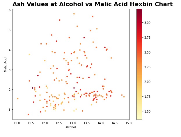
Below, we have created one more example showing distribution of third ingredient ash based on values of alcohol and malic acid.
import matplotlib.pyplot as plt

plt.figure(figsize=(9,7))

plt.hexbin(wine_df["alcohol"], wine_df["malic_acid"], wine_df["ash"], cmap="YlOrRd")

plt.colorbar()

plt.xlabel("Alcohol")
plt.ylabel("Malic Acid")

plt.title("Ash Values at Alcohol vs Malic Acid Hexbin Chart", loc="left", fontdict=dict(fontsize=20, fontweight="bold"), pad=10)

plt.show()
12. Styling Charts (Improve Chart Look & Feel Easily using Themes) 
Now, you noticed that all our previous charts look quite simple. There is no background color or grid or any other aesthetics to improve look of charts. We can add those things manually but that will require us to code more.
We can avoid more coding by selecting one of the ready-made themes available from matplotlib for our purpose. Matplotlib provides themes used by famous libraries and blogs like seaborn, ggplot, and fivethirtyeight.
In this section, we have explained two different ways of using these themes for our chart.
Below is the first way of specifying theme. We can specify theme using context() function available from style sub-module of matplotlib. We need to use it as context manager and the theme will be used for code inside of that context only.
This is very useful when you want to use theme for particular charts only.
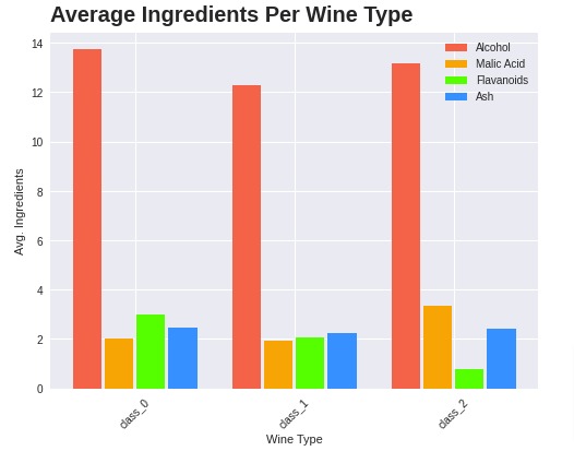
We have added seaborn theme to our grouped bar chart that we had created earlier.
import matplotlib
import matplotlib.pyplot as plt

with matplotlib.style.context("seaborn"):
    plt.figure(figsize=(8,6))

    plt.bar(x=[0,5,10], height=avg_wine_df["alcohol"], width=0.9, color="tomato", label="Alcohol")
    plt.bar(x=[1,6,11], height=avg_wine_df["malic_acid"], width=0.9, color="orange", label="Malic Acid")
    plt.bar(x=[2,7,12], height=avg_wine_df["flavanoids"], width=0.9, color="lime", label="Flavanoids")
    plt.bar(x=[3,8,13], height=avg_wine_df["ash"], width=0.9, color="dodgerblue", label="Ash")

    ## Set Axes Labels
    plt.xlabel("Wine Type")
    plt.ylabel("Avg. Ingredients")

    plt.xticks(ticks=[1.5, 6.5, 11.5], labels=avg_wine_df["WineType"], rotation=45)

    plt.title("Average Ingredients Per Wine Type", loc="left", fontdict=dict(fontsize=20, fontweight="bold"), pad=10)

    plt.legend(loc='best')

    plt.show()
We can retrieve names of available themes using available attribute of style sub-module of pyplot.
print("List of Available Styles : {}".format(plt.style.available))
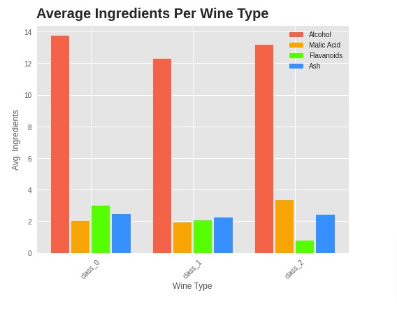
Below, we have created one more example demonstrating use of context() function.
import matplotlib
import matplotlib.pyplot as plt

with matplotlib.style.context(("seaborn", "ggplot") ):
    plt.figure(figsize=(8,6))

    plt.bar(x=[0,5,10], height=avg_wine_df["alcohol"], width=0.9, color="tomato", label="Alcohol")
    plt.bar(x=[1,6,11], height=avg_wine_df["malic_acid"], width=0.9, color="orange", label="Malic Acid")
    plt.bar(x=[2,7,12], height=avg_wine_df["flavanoids"], width=0.9, color="lime", label="Flavanoids")
    plt.bar(x=[3,8,13], height=avg_wine_df["ash"], width=0.9, color="dodgerblue", label="Ash")

    ## Set Axes Labels
    plt.xlabel("Wine Type")
    plt.ylabel("Avg. Ingredients")

    plt.xticks(ticks=[1.5, 6.5, 11.5], labels=avg_wine_df["WineType"], rotation=45)

    plt.title("Average Ingredients Per Wine Type", loc="left", fontdict=dict(fontsize=20, fontweight="bold"), pad=10)

    plt.legend(loc='best')

    plt.show()
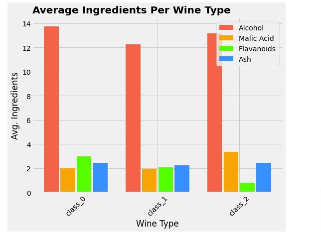
Below, we have explained second way of specifying theme for our chart. We can use use() function available from style sub-module of pyplot. We need to provide theme name for it.
This will permanently set theme and all upcoming charts will use this theme.
import matplotlib.pyplot as plt

plt.style.use("fivethirtyeight")

plt.figure(figsize=(8,6))

plt.bar(x=[0,5,10], height=avg_wine_df["alcohol"], width=0.9, color="tomato", label="Alcohol")
plt.bar(x=[1,6,11], height=avg_wine_df["malic_acid"], width=0.9, color="orange", label="Malic Acid")
plt.bar(x=[2,7,12], height=avg_wine_df["flavanoids"], width=0.9, color="lime", label="Flavanoids")
plt.bar(x=[3,8,13], height=avg_wine_df["ash"], width=0.9, color="dodgerblue", label="Ash")

## Set Axes Labels
plt.xlabel("Wine Type")
plt.ylabel("Avg. Ingredients")

plt.xticks(ticks=[1.5, 6.5, 11.5], labels=avg_wine_df["WineType"], rotation=45)

plt.title("Average Ingredients Per Wine Type", loc="left", fontdict=dict(fontsize=20, fontweight="bold"), pad=10)

plt.legend(loc='best')

plt.show()
 Sunny Solanki
Sunny Solanki
Intro: Software Developer | Youtuber | Bonsai Enthusiast
About: Sunny Solanki holds a bachelor's degree in Information Technology (2006-2010) from L.D. College of Engineering. Post completion of his graduation, he has 8.5+ years of experience (2011-2019) in the IT Industry (TCS). His IT experience involves working on Python & Java Projects with US/Canada banking clients. Since 2020, he’s primarily concentrating on growing CoderzColumn.
His main areas of interest are AI, Machine Learning, Data Visualization, and Concurrent Programming. He has good hands-on with Python and its ecosystem libraries.
Apart from his tech life, he prefers reading biographies and autobiographies. And yes, he spends his leisure time taking care of his plants and a few pre-Bonsai trees.
Contact: sunny.2309@yahoo.in


![YouTube Subscribe]() Comfortable Learning through Video Tutorials?
Comfortable Learning through Video Tutorials?
If you are more comfortable learning through video tutorials then we would recommend that you subscribe to our YouTube channel.
![Need Help]() Stuck Somewhere? Need Help with Coding? Have Doubts About the Topic/Code?
Stuck Somewhere? Need Help with Coding? Have Doubts About the Topic/Code?
 Stuck Somewhere? Need Help with Coding? Have Doubts About the Topic/Code?
When going through coding examples, it's quite common to have doubts and errors.
If you have doubts about some code examples or are stuck somewhere when trying our code, send us an email at coderzcolumn07@gmail.com. We'll help you or point you in the direction where you can find a solution to your problem.
You can even send us a mail if you are trying something new and need guidance regarding coding. We'll try to respond as soon as possible.
![Share Views]() Want to Share Your Views? Have Any Suggestions?
Want to Share Your Views? Have Any Suggestions?
 Want to Share Your Views? Have Any Suggestions?
If you want to
- provide some suggestions on topic
- share your views
- include some details in tutorial
- suggest some new topics on which we should create tutorials/blogs
 datascience, datavisulisation, matplotlib