How to Create Sankey Diagrams (Alluvial) in Python [holoviews & plotly]?
What is Sankey Diagram?
Sankey Diagram is used to display the flow of some property from various sources to destinations.
The simple diagram has a few source nodes plotted at the beginning and a few destination nodes at the end of the diagram. Then, there are various arrows/links representing the flow of property from sources to destinations. There is one arrow/link per source and destination combination. The width of an arrow/link is proportional to the amount of property flowing from source to destination.
The Sankey diagrams can have intermediate nodes (plotted between source and destination nodes) as well when the path from source to destination involves multiple intermediate nodes (E.g., Journey of users on website pages).
Applications of Sankey Diagram
Sankey diagrams and its variation like Alluvial Diagrams are commonly used for purposes like analyzing population migration, website user journey, the flow of energy, the flow of other properties (oil, gas, etc.), research paper citations, etc. Google Analytics uses an alluvial diagram to show users' Journey on a website (sessions).
Nowadays Python is the most preferred library for data analysis and visualization hence we'll try to create Sankey diagrams using Python data visualization libraries.
What can you learn from this article?
As a part of this article, we have explained how to create a Sankey Diagram (Alluvial Diagram) in Python using libraries holoviews and plotly. The charts created using both libraries are interactive. Apart from plotting simple Sankey diagrams, we have also explained various ways to style the plot and improve its aesthetics (look & feel).
Holoviews is a high-level library that let us specify chart metadata and then creates charts using one of its back end (Bokeh, Matplotlib or Plotly). It takes pandas dataframe as a dataset and lets us create charts from it.
Plotly is an independent data visualization library with extensive support for many chart types. The dataset used to create various Sankey Diagrams has Population migration data from New Zealand.
Please make a NOTE that all diagrams are created in Jupyter Notebook.
If you are someone who is new to holoviews and want to learn about it then we would recommend that you go through our simple tutorial on it in your free time.
Below, we have listed important sections of the Tutorial to give an overview of the material covered.
Important Sections Of Tutorial
- Prepare Dataset
- Sankey Diagram Using "Holoviews"
- 1.1 Population Migration between "New Zealand" & Various "Continents"
- 1.2 Population Migration between "New Zealand" & Various "European Countries"
- 1.3 Depict Users Journey on a Website
- Sankey Diagram using "Plotly"
- 2.1 Population Migration between "New Zealand" & Various "Continents"
- 2.2 Population Migration between "New Zealand" & Various "European Countries"
- 2.3 Users' Journey on a Website
This ends our small introduction to the tutorial. So without further delay, let's get started with the coding part.
Below we have first imported the necessary Python libraries and printed the versions that we have used in our tutorial.
import pandas as pd
import numpy as np
import holoviews as hv

print("Holoviews Version : {}".format(hv.__version__))
import plotly

print("Plotly Version : {}".format(plotly.__version__))
0. Prepare Dataset 
Load Dataset
We'll be using the New Zealand migration dataset for our plotting purpose. It's available on kaggle for download.
Dataset Details
Dataset has information about a number of people who departed from and arrived in New Zealand from all continents and countries of the world from 1979 till 2016. We'll be aggregating this data in various ways to create different Sankey diagrams. We suggest that you download this dataset to follow along with us.
Below, We have loaded the dataset as a pandas dataframe.
nz_migration = pd.read_csv("~/datasets/migration_nz.csv")

nz_migration.head()
Prepare Dataset By Cleaning and Aggregating Entries
After loading the dataset, we have performed a few steps of data cleaning and aggregation as mentioned below.
- We'll remove entries other than arrival and departure.
- We'll remove entries where the proper country name is not present.
- We'll then group the dataframe by Measure & Country attributes and sum up all entries.
After performing the above steps, we'll have a dataset where we'll have information about arrivals and departure counts from each country and continent of all time.
nz_migration = nz_migration[nz_migration["Measure"]!="Net"] ## Removing Entries related to "Net Total"
nz_migration = nz_migration[~nz_migration["Country"].isin(["Not stated", "All countries"])] ## Removing entries with No Details or all countries

nz_migration_grouped = nz_migration.groupby(by=["Measure","Country"]).sum()[["Value"]]
nz_migration_grouped = nz_migration_grouped.reset_index()

nz_migration_grouped.head(10) ## Displaying first 10 rows
1. Sankey Diagrams Using "Holoviews" 
In this section, we have plotted different Sankey Diagrams using holoviews as our plotting library. The charts created using Holoviews are interactive. We can hover over a link to check the amount of flow of property which will be displayed in a tooltip. It even displays source and destination node names.
Below, We have set the backend of holoviews as bokeh first. It'll now create charts using it.
hv.extension('bokeh')

1.1 Population Migration between "New Zealand" & Various "Continents"
For our first Sankey diagram, we need to filter entries of the dataframe to keep only entries where the count for each continent is present. Below we are filtering the dataset based on continent names to remove all other entries.
continents = ["Asia", "Australia","Africa and the Middle East","Europe", "Americas", "Oceania"]

continent_wise_migration = nz_migration_grouped[nz_migration_grouped.Country.isin(continents)]

continent_wise_migration
1.1.1 Simple Sankey Diagram
We can plot a Sankey diagram very easily using holoviews by passing it above the dataframe. Holoviews needs a dataframe with at least three columns. It'll consider the first column as source, the second as destination, and the third as property flow value from source to destination. It'll plot links between each combination of source and destination.
hv.Sankey(continent_wise_migration)
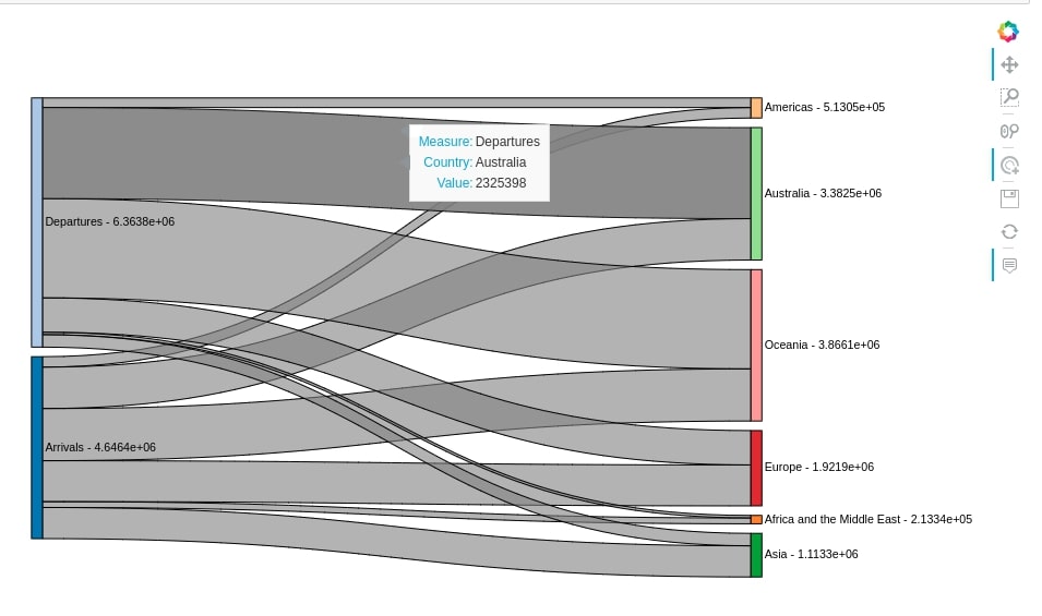
We can notice from the above chart that all links have a gray color. We can color them in two ways.
- Source Node Color - It'll color links with the same color as the source node from which they originated. This helps us better understand the flow from source to destination.
- Destination Node Color - It'll color links with the same color as the destination node to which they are going. This helps us better understand reverse flow from destination to source.
You can color links according to your need. We have explained in our tutorial how we can color links using both ways.
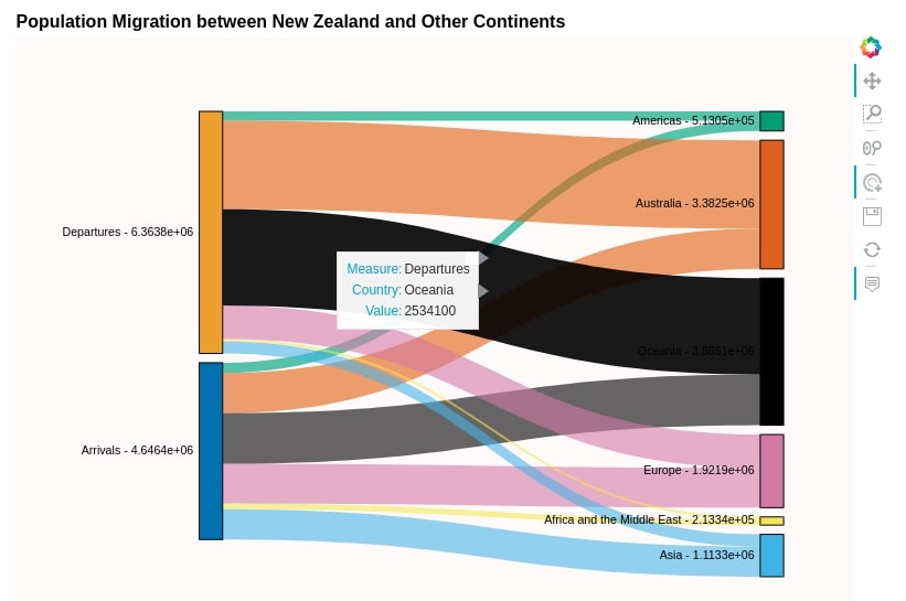
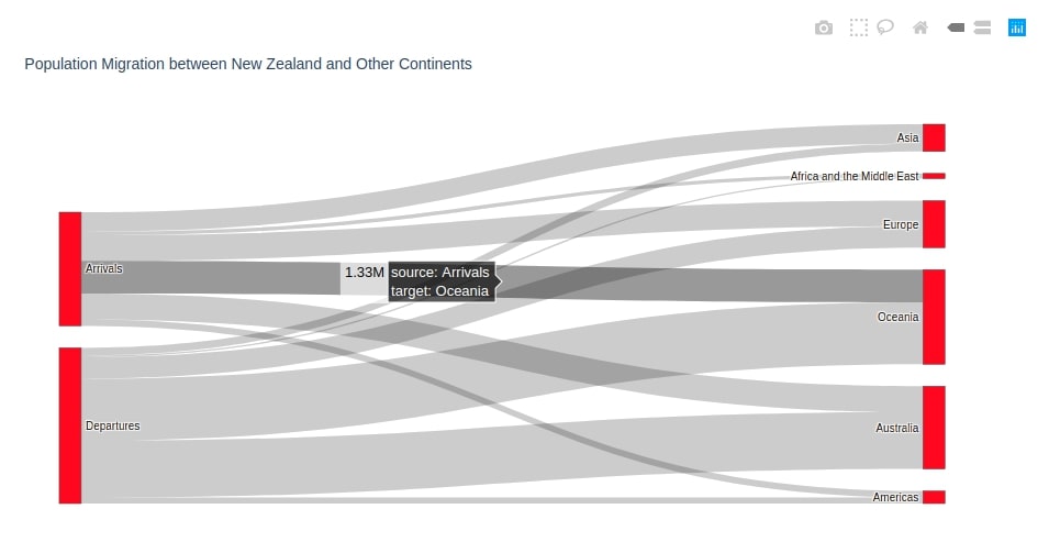
1.1.2 Coloring Edges as Per Destination Node Color
Below we are creating the same Sankey plot again, but this time specifying which columns from the dataframe to take as source and destination in kdims parameter and which column to use to generate property flow arrow sizes using vdims parameter.
We have also specified various parameters as a part of opts() method called on the Sankey plot object which helped us further improve the styling of the diagram further.
We have included colormap to use for nodes & edges, label position in the diagram, column to use for edge color, edge line width, node opacity, graph width & height, graph background color, and title attributes which improves the styling of the graph a lot and makes it aesthetically pleasing.
## Providing column names to use as Source, Destination and Flow Value.
sankey1 = hv.Sankey(continent_wise_migration, kdims=["Measure", "Country"], vdims=["Value"])

## Modifying Default Chart Options
sankey1.opts(cmap='Colorblind',
             label_position='left',
             edge_color='Country', edge_line_width=0,
             node_alpha=1.0, node_width=40, node_sort=True,
             width=800, height=600, bgcolor="snow",
             title="Population Migration between New Zealand and Other Continents")
1.1.3 Specifying Chart Options using Jupyter Notebook Magic Command ("%%opts")
Below, we have created the same Sankey Diagram as the previous cell but this time we have specified chart options using '%%opts' magic command of Jupyter Notebook.
Please make a NOTE that options to modify chart aesthetics are provided in parenthesis and options to modify chart are provided in brackets. You can retrieve other option names by pressing Tab inside of brackets or parenthesis.
If you are someone who is not aware of Jupyter notebook magic commands and want to learn about them then do check the below link. It covers the majority of them in detail.
%%opts Sankey [width=800, height=600 bgcolor="snow" title="Population Migration between New Zealand and Other Continents"]
%%opts Sankey [label_position="left" node_sort=True node_width=40]
%%opts Sankey (cmap="Colorblind" edge_color='Country' edge_line_width=0 node_alpha=1.0)

sankey1 = hv.Sankey(continent_wise_migration, kdims=["Measure", "Country"], vdims=["Value"])

sankey1
After going through the above chart, we can see that majority of people departed to Australia, Oceania, and Europe from New Zealand whereas many people arrive in New Zealand from Oceania, Europe, Australia, and Asia. There is very less departure to Asia and Africa from New Zealand. We also noticed that migration to and from the Americas is also quite less compared to other continents.
1.2 Population Migration between New Zealand & Various European Countries 
We'll now try to plot another Sankey Diagram depicting population migration between New Zealand and various European countries.
For plotting that, we first need to filter our dataframe keeping entry for only European countries.
NOTE
Please make a note that we have not kept all European countries as few countries had very less migration history with New Zealand and thus have been excluded to prevent the graph from getting messy as it was not giving much information.
european_countries = ['Austria', 'Belgium', 'Bulgaria', 'Croatia', 'Denmark', 'Finland', 'France',
                      'Germany', 'Greece', 'Ireland', 'Italy', 'Netherlands', 'Norway', 'Poland',
                      'Romania', 'Russia', 'Spain', 'Sweden', 'Switzerland', 'Ukraine']

european_countries_migration = nz_migration_grouped[nz_migration_grouped["Country"].isin(european_countries)]

european_countries_migration.head()
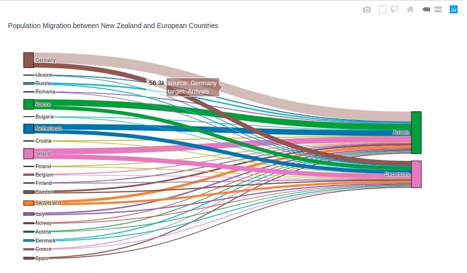
1.2.1 Coloring Edges as Per Source Node Colors
We are plotting below our third Sankey Diagram showing population flow between New Zealand and European countries.
Please make a note that we have changed the source and target attributes this time by reversing them from the previous one. We have also modified various styling attributes but this time we have modified them using the jupyter notebook magic command. This is another way to modify styling and various other graph attributes of holoviews graphs as explained earlier.
TIP
You can try styling and other graph configuration attributes available with holoviews by pressing Tab between parenthesis and brackets. It'll suggest you a list of attributes available for that graph by showing the list but you need to specify the graph name after %%opts magic command for it to work.
%%opts Sankey (cmap='Category10' edge_color='Measure' edge_line_width=0 node_alpha=1.0)
%%opts Sankey [node_sort=False label_position='left' bgcolor="snow" node_width=40 node_sort=True ]
%%opts Sankey [width=900 height=800 title="Population Migration between New Zealand and European Countries"]
%%opts Sankey [margin=0 padding=0]

hv.Sankey(european_countries_migration, kdims=["Measure", "Country"], vdims=["Value"])
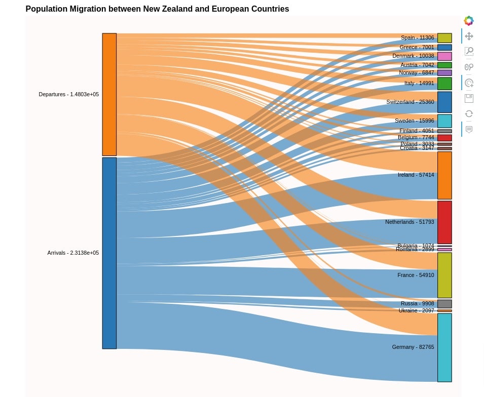
We can see from the above graph that countries like Germany, France, Netherlands, Ireland, and Switzerland have a very high flow of population migration with New Zealand. A lot of peoples arrives in New Zealand from these countries.
NOTE
Please make a note that it's advisable to limit number of entries in graph to prevent it from getting cluttered. We can see that the above graph looks a bit cluttered. One can remove entries that are less significant or have less value to properly highlight other more significant values.
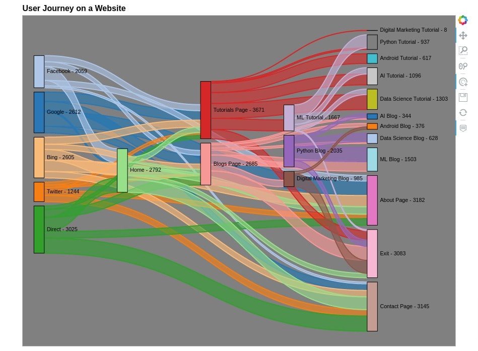
1.3 Users Journey on a Website 
Our third Sankey Diagram will have more than 2 layers (Intermediate Nodes). We'll now try to display the journey of a user on our website by simulating user flow between major pages of our website. Below we are first creating a dataset about the flow of a number of users between various pages of our website.
source_dest = [
    ["Google", "Home"],
    ["Google", "Tutorials Page"],
    ["Google", "Blogs Page"],
    ["Google", "Contact Page"],
    ["Google", "About Page"],

    ["Facebook", "Home"],
    ["Facebook", "Tutorials Page"],
    ["Facebook", "Blogs Page"],
    ["Facebook", "Contact Page"],
    ["Facebook", "About Page"],

    ["Twitter", "Home"],
    ["Twitter", "Tutorials Page"],
    ["Twitter", "Blogs Page"],
    ["Twitter", "Contact Page"],
    ["Twitter", "About Page"],

    ["Bing", "Home"],
    ["Bing", "Tutorials Page"],
    ["Bing", "Blogs Page"],
    ["Bing", "Contact Page"],
    ["Bing", "About Page"],

    ["Direct", "Home"],
    ["Direct", "Tutorials Page"],
    ["Direct", "Blogs Page"],
    ["Direct", "Contact Page"],
    ["Direct", "About Page"],

    ["Home", "Exit"],
    ["Home", "Tutorials Page"],
    ["Home", "Blogs Page"],
    ["Home", "Contact Page"],
    ["Home", "About Page"],

    ["Tutorials Page", "Exit"],
    ["Tutorials Page", "Python Tutorial"],
    ["Tutorials Page", "ML Tutorial"],
    ["Tutorials Page", "AI Tutorial"],
    ["Tutorials Page", "Data Science Tutorial"],
    ["Tutorials Page", "Digital Marketing Tutorial"],
    ["Tutorials Page", "Android Tutorial"],

    ["Blogs Page", "Exit"],
    ["Blogs Page", "Python Blog"],
    ["Blogs Page", "ML Blog"],
    ["Blogs Page", "AI Blog"],
    ["Blogs Page", "Data Science Blog"],
    ["Blogs Page", "Digital Marketing Blog"],
    ["Blogs Page", "Android Blog"],

    ["Python Blog", "Exit"],
    ["Python Blog", "ML Blog"],
    ["Python Blog", "AI Blog"],
    ["Python Blog", "Data Science Blog"],

    ["ML Tutorial", "Python Tutorial"],
    ["ML Tutorial", "Exit"],
    ["ML Tutorial", "AI Tutorial"],
    ["ML Tutorial", "Data Science Tutorial"],

    ["Digital Marketing Blog", "Exit"],
    ["Digital Marketing Blog", "Android Blog"],
]

website_vists = pd.DataFrame(source_dest, columns=["Source", "Dest"])
website_vists["Count"] = np.random.randint(1,1000, size=website_vists.shape[0])
website_vists.head()
Below we are creating our third Sankey Diagram showing the journey of users on our website based on simulated data create above. We also have modified various styling and graph configuration attributes to improve its aesthetics.
%%opts Sankey (edge_color="Source"  edge_line_width=2 node_cmap="tab20")
%%opts Sankey (node_alpha=1.0 edge_hover_fill_color="red")
%%opts Sankey [node_sort=False label_position='right' node_width=30 node_sort=True ]
%%opts Sankey [title="User Journey on a Website" width=900 height=700]
%%opts Sankey [margin=0 padding=0 bgcolor="grey"]

hv.Sankey(website_vists, kdims=["Source", "Dest"], vdims=["Count"])
2. Sankey Diagram using "Plotly" 
In this section, we have explained different ways to generate Sankey Diagram using the Python library Plotly. We have tried to recreate the same diagrams as Holoviews section but using Plotly this time. The charts created using Plotly are interactive. We can hover over links to check the amount of flow of property which will be displayed in a tooltip along with source and target names.
2.1 Population Migration between New Zealand & Various Continents 
The process of generating a Sankey Diagram using Plotly is a bit different from holoviews and requires a bit of data processing before actually plotting the graph.
Plotly requires that we provide it a list of node names and indexes of source & destination nodes along with flow value separately.
Steps to Create Sankey Diagram using "Plotly"
Below, we have listed steps that we need to perform in order to generate Sankey Diagrams using plotly.
- First, we'll need to create a list of all possible nodes.
- Then We need to generate an index list of source nodes and target nodes based on their index in the list of all nodes created in previous steps.
- We then need to pass all possible nodes to node parameter of Sankey() method of graph_objects module as explained below.
- We pass all source and destination indices as well as flow value between that nodes to link parameter of Sankey() method of graph_objects plotly module as per the below example.
- We can then update various plot attributes by using update_layout() method on a figure object.
Please don't worry if you don't understand steps fully. Go ahead with code as it'll become clear when you execute code. You can analyze individual variables to see what they are holding to better understand the process.
import plotly.graph_objects as go
import plotly.express as pex
2.1.1 Uncolored Nodes & Links
## All chart nodes
all_nodes = continent_wise_migration.Measure.values.tolist() + continent_wise_migration.Country.values.tolist()

## Indices of sources and destinations
source_indices = [all_nodes.index(measure) for measure in continent_wise_migration.Measure] ## Retrieve source nodes indexes as per all nodes list.
target_indices = [all_nodes.index(country) for country in continent_wise_migration.Country] ## Retrieve destination nodes indexes as per all nodes list.

fig = go.Figure(data=[go.Sankey(
                        # Define nodes
                        node = dict(
                          label =  all_nodes,
                          color =  "red"
                        ),

                        # Add links
                        link = dict(
                          source =  source_indices,
                          target =  target_indices,
                          value =  continent_wise_migration.Value,
                        )
                    )
                ])

fig.update_layout(title_text="Population Migration between New Zealand and Other Continents",
                  font_size=10)
fig.show()
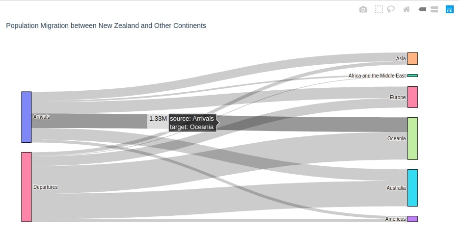
2.1.2 Colored Nodes & Uncolored Links
The above graph used red color as a default color for all nodes. We can omit that attribute and plotly will use its default colors for different nodes of the graph.
all_nodes = continent_wise_migration.Measure.values.tolist() + continent_wise_migration.Country.values.tolist()

source_indices = [all_nodes.index(measure) for measure in continent_wise_migration.Measure] ## Retrieve source nodes indexes as per all nodes list.
target_indices = [all_nodes.index(country) for country in continent_wise_migration.Country] ## Retrieve destination nodes indexes as per all nodes list.


fig = go.Figure(data=[go.Sankey(
                        node = dict(
                              pad = 20,
                              thickness = 20,
                              line = dict(color = "black", width = 1.0),
                              label =  all_nodes,
                        ),

                        link = dict(
                              source =  source_indices,
                              target =  target_indices,
                              value =  continent_wise_migration.Value,
                        )
                    )
                ])

fig.update_layout(title_text="Population Migration between New Zealand and Other Continents",
                  font_size=10)
fig.show()
2.2 Population Migration between New Zealand & Various European Countries 
Below we are plotting the second Sankey Diagram using plotly.
We have this time introduced logic to color various nodes and links of the diagram. We are maintaining a dictionary of mapping from node name to color. We are then using this dictionary to specify the color of nodes and edges. We have used D3 color palette to select colors for nodes.
We suggest that you try various combinations of colors and use different colors for nodes and edges to show them differently.
all_nodes = european_countries_migration.Country.values.tolist() + european_countries_migration.Measure.values.tolist()

source_indices = [all_nodes.index(country) for country in european_countries_migration.Country] ## Retrieve source nodes indexes as per all nodes list.
target_indices = [all_nodes.index(measure) for measure in european_countries_migration.Measure] ## Retrieve destination nodes indexes as per all nodes list.

colors = pex.colors.qualitative.D3 ## Color Pallete

node_colors_mappings = dict([(node,np.random.choice(colors)) for node in all_nodes]) ## Node to Color Mapping

node_colors = [node_colors_mappings[node] for node in all_nodes] ## Node Colors
edge_colors = [node_colors_mappings[node] for node in european_countries_migration.Country] ## Color Links according to Country Nodes

fig = go.Figure(data=[
                    go.Sankey(
                        node = dict(
                                  pad = 20,
                                  thickness = 20,
                                  line = dict(color = "black", width = 1.0),
                                  label =  all_nodes,
                                  color =  node_colors, ## Node Colors
                                ),

                        link = dict(
                              source =  source_indices,
                              target =  target_indices,
                              value =  european_countries_migration.Value,
                              color = edge_colors, ## Link Colors
                              )
                            )
                        ])

fig.update_layout(title_text="Population Migration between New Zealand and European Countries",
                  height=600,
                  font_size=10)
fig.show()
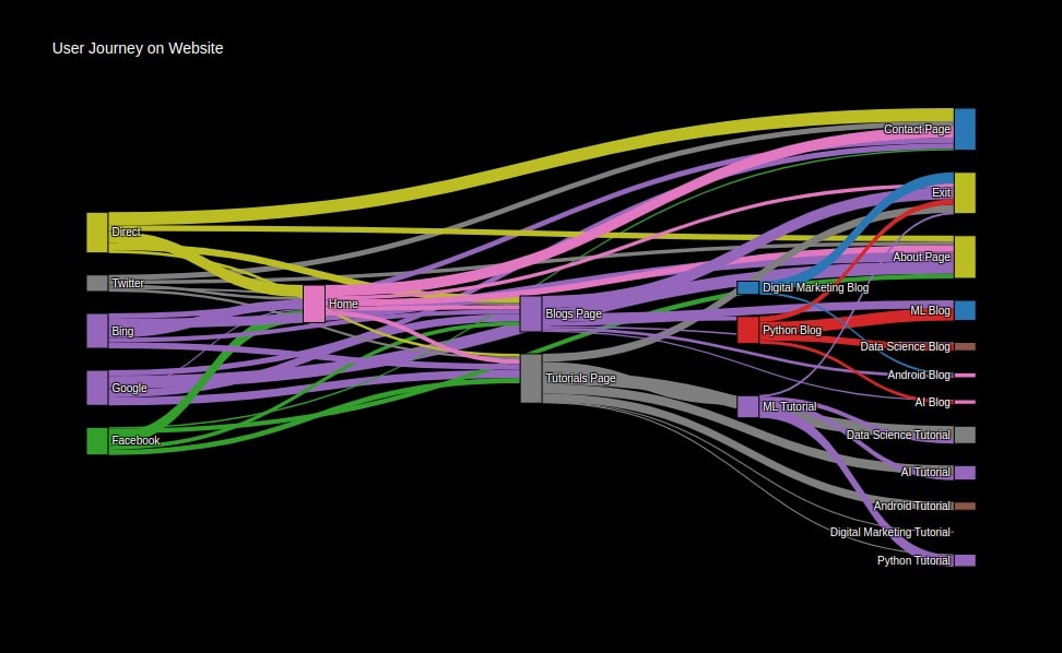
2.3 Users Journey on a Website 
We are again generating Sankey Diagram representing the user journey on a website that we had generated above but this time using plotly. We have also tried to improve the look of the graph by modifying its background and other configuration attributes.
all_nodes = website_vists.Source.values.tolist() + website_vists.Dest.values.tolist()

source_indices = [all_nodes.index(source) for source in website_vists.Source] ## Retrieve source nodes indexes as per all nodes list.
target_indices = [all_nodes.index(dest) for dest in website_vists.Dest] ## Retrieve destination nodes indexes as per all nodes list.

colors = pex.colors.qualitative.D3

node_colors_mappings = dict([(node,np.random.choice(colors)) for node in all_nodes])

node_colors = [node_colors_mappings[node] for node in all_nodes]
edge_colors = [node_colors_mappings[node] for node in website_vists.Source] ## Color links according to source nodes

fig = go.Figure(data=[
                    go.Sankey(
                        node = dict(
                                pad = 20,
                                thickness = 20,
                                line = dict(color = "black", width = 1.0),
                                label =  all_nodes,
                                color =  node_colors,
                               ),
                        link = dict(
                               source =  source_indices,
                               target =  target_indices,
                               value =  website_vists.Count,
                               color = edge_colors
                               )
                         )
                    ])

fig.update_layout(title_text="User Journey on Website",
                  height=600,
                  font=dict(size = 10, color = 'white'),
                  plot_bgcolor='black', paper_bgcolor='black')

fig.show()
This ends our small tutorial explaining how to plot Sankey Diagram in Python using data visualization libraries holoviews and plotly.
References 
 Sunny Solanki
Sunny Solanki
Intro: Software Developer | Youtuber | Bonsai Enthusiast
About: Sunny Solanki holds a bachelor's degree in Information Technology (2006-2010) from L.D. College of Engineering. Post completion of his graduation, he has 8.5+ years of experience (2011-2019) in the IT Industry (TCS). His IT experience involves working on Python & Java Projects with US/Canada banking clients. Since 2020, he’s primarily concentrating on growing CoderzColumn.
His main areas of interest are AI, Machine Learning, Data Visualization, and Concurrent Programming. He has good hands-on with Python and its ecosystem libraries.
Apart from his tech life, he prefers reading biographies and autobiographies. And yes, he spends his leisure time taking care of his plants and a few pre-Bonsai trees.
Contact: sunny.2309@yahoo.in


![YouTube Subscribe]() Comfortable Learning through Video Tutorials?
Comfortable Learning through Video Tutorials?
If you are more comfortable learning through video tutorials then we would recommend that you subscribe to our YouTube channel.
![Need Help]() Stuck Somewhere? Need Help with Coding? Have Doubts About the Topic/Code?
Stuck Somewhere? Need Help with Coding? Have Doubts About the Topic/Code?
 Stuck Somewhere? Need Help with Coding? Have Doubts About the Topic/Code?
When going through coding examples, it's quite common to have doubts and errors.
If you have doubts about some code examples or are stuck somewhere when trying our code, send us an email at coderzcolumn07@gmail.com. We'll help you or point you in the direction where you can find a solution to your problem.
You can even send us a mail if you are trying something new and need guidance regarding coding. We'll try to respond as soon as possible.
![Share Views]() Want to Share Your Views? Have Any Suggestions?
Want to Share Your Views? Have Any Suggestions?
 Want to Share Your Views? Have Any Suggestions?
If you want to
- provide some suggestions on topic
- share your views
- include some details in tutorial
- suggest some new topics on which we should create tutorials/blogs
 sankey-diagram, holoviews, plotly