Updated On : Aug-27,2022 Time Investment : ~30 mins

How to Remove Trend & Seasonality from Time-Series Data [Python]?¶

Both Trends and Seasonality are generally present in the majority of time series data of the real world. When we want to do the forecasting with time series, we need a stationary time series.

The stationary time series is time-series dataset where there is no trend or seasonality information present in it. The stationary time series is a series with constant mean, constant variance, and constant autocorrelation.

To make time series stationary, we need to find a way to remove trends and seasonality from our time series so that we can use it with prediction models. To do that, we need to understand what is trends and seasonality in-depth to handle them better.

Apart from trend and seasonality, some time-series also have noise/error/residual component present as well. We can decompose time-series to see different components.

> What Can You Learn From This Article?¶

As a part of this tutorial, we have explained how to detect and then remove trend as well as seasonality present in time-series dataset. We have explained different ways to remove trend & seasonality like power transformation, log transformation, moving window function, linear regression, etc from data. Apart from this, we have also explained how to test for stationarity once trend & seasonality are removed. Tutorial is a good starting point for understanding concepts like trend, seasonality, stationarity, etc.

Below, we have listed important sections of Tutorial to give an overview of the material covered.

Important Sections Of Tutorial¶

Types of Time-Series
What is Trend?
- Ways to Remove Trend
What is Seasonality
- Ways to Remove Seasonality
Load Dataset For Tutorial
Decompose Time-Series to See Individual Components
Checking Whether Time-Series is Stationary or Not
- Stationarity Check By Calculating Change in Mean, Variance & Auto-Covariance Over Time
- Stationarity Check using ACF Plot
- Dicky-Fuller Test for Stationarity
Remove Trend
- Logged Transformation
- Power Transformations
- Moving Window Functions
- Linear Regression to Remove Trend
Remove Seasonality
- Differencing Over Log Transformed Time-Series
  - Test for Stationarity
- Differencing Over Power Transformed Time-Series
- Differencing Over Linear Regression Transformed Time-Series

1. Types of Time-Series ¶

Time-series are of generally two types:

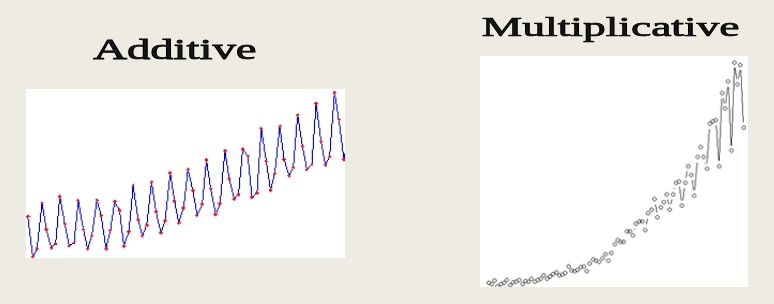
Additive Time-Series: Additive time-series is time-series where components (trend, seasonality, noise) are added to generate time series.
- Time-Series = trend + seasonality + noise
Multiplicative Time-Series: Multiplicative time-series is time-series where components (trend, seasonality, noise) are multiplied to generate time series. one can notice an increase in the amplitude of seasonality in multiplicative time-series.
- Time-Series = trend seasonality noise

2. Trend ¶

The trend represent an increase or decrease in time-series value over time. If we notice that the value of measurement over time is increasing or decreasing then we can say that it has an upward or downward trend.

How to remove trend from time-series data?¶

There are various ways to de-trend a time series. We have explained a few below.

Log Transformation.
Power Transformation.
local smoothing - Applying moving window functions to time-series data.
Differencing a time-series.
Linear Regression.

3. Seasonality ¶

The seasonality represents variations in measured value which repeats over the same time interval regularly. If we notice that particular variations in value are happening every week, month, quarter or half-yearly then we can say that time series has some kind of seasonality.

How to remove seasonality from time-series data?¶

There are various ways to remove seasonality. The task of removing seasonality is a bit complicated. We have explained a few ways below to remove seasonality.

Average de-trended values.
Differencing a time-series.
Use the loess method.

4. Load Time Series Dataset ¶

We'll now explore trend and seasonality removal with examples. We'll be using famous air passenger datasets available on-line for our purpose because it has both trend and seasonality. It has information about US airline passengers from 1949 to 1960 recorded each month. Please download the dataset to follow along.

Air Passengers Dataset

import pandas as pd
import numpy as np
import matplotlib.pyplot as plt

%matplotlib inline

air_passengers = pd.read_csv("~/datasets/AirPassengers.csv", index_col=0, parse_dates=True)
air_passengers.head()

	#Passengers
Month
1949-01-01	112
1949-02-01	118
1949-03-01	132
1949-04-01	129
1949-05-01	121

air_passengers.plot(figsize=(8,4), color="tab:red");

air_passengers["1952"].plot(kind="bar", color="tab:green", legend=False);

By looking at the above plots we can see that our time-series is multiplicative time-series and has both trend as well as seasonality. We can see the trend as passengers are constantly increasing over time. We can see seasonality with the same variations repeating for 1 year where value peaks somewhere are around August.

5. Decompose Time-Series to See Components (Trend, Seasonality, Noise, etc)¶

We can decompose time-series to see various components of time-series. Python module named statmodels provides us with easy to use utility which we can use to get an individual component of time-series and then visualize it.

from statsmodels.tsa.seasonal import seasonal_decompose

decompose_result = seasonal_decompose(air_passengers, model="multiplicative")

trend = decompose_result.trend
seasonal = decompose_result.seasonal
residual = decompose_result.resid

decompose_result.plot();

We can notice trend and seasonality components separately as well as residual components. There is a loss of residual in the beginning which is settling later.

6. Checking Whether Time-Series is Stationary or Not ¶

As we declared above time-series is stationary whose mean, variance and auto-covariance are independent of time. We can check mean, variance and auto-covariance using moving window functions available with pandas. We'll also use a dicky-fuller test available with statsmodels to check the stationarity of time-series. If time-series is not stationary then we need to make it stationary.

Below we have taken an average over moving window of 12 samples. We noticed from the above plots that there is the seasonality of 12 months in time-series. We can try different window sizes for testing purposes.

air_passengers.rolling(window = 12).mean().plot(figsize=(8,4), color="tab:red", title="Rolling Mean over 12 month period");

air_passengers.rolling(window = 20).mean().plot(figsize=(8,4), color="tab:red", title="Rolling mean over 20 month period");

We can clearly see that time-series has a visible upward trend.

Below we have taken variance over the moving window of 12 samples. We noticed from the above plots that there is the seasonality of 12 months in time-series.

air_passengers.rolling(window = 12).var().plot(figsize=(8,4), color="tab:red", title="Rolling Variance over 12 month period");

air_passengers.rolling(window = 20).var().plot(figsize=(8,4), color="tab:red", title="Rolling variance over 20 month period");

From the above two plots, we notice that time series has some kind of multiplicative effect which seems to be increasing with time period. We can see the low seasonality effect at the beginning which amplifies over time.

Below we are also plotting an auto-correlation plot for time-series data as well. This plot helps us understand whether present values of time series are positively correlated, negatively correlated, or not related at all to past values. statsmodels library provides ready to use method plot_acf as a part of module statsmodels.graphics.tsaplots.

from statsmodels.graphics.tsaplots import plot_acf


plot_acf(air_passengers);

We can notice from the above chart that after 13 lags, the line gets inside confidence interval (light blue area). This can be due to seasonality of 12-13 months in our data.

Dicky-Fuller Test for Stationarity¶

Once we have removed trend and seasonality from time-series data then we can test its stationarity using a dicky-fuller test. It's a statistical test to check the stationarity of time-series data.

Further Read About Test

We can perform Dicky-Fuller test functionality available with the statsmodels library.

Below we'll test the stationarity of our time-series with this functionality and try to interpret its results to better understand it.

from statsmodels.tsa.stattools import adfuller

dftest = adfuller(air_passengers['#Passengers'], autolag = 'AIC')

print("1. ADF : ",dftest[0])
print("2. P-Value : ", dftest[1])
print("3. Num Of Lags : ", dftest[2])
print("4. Num Of Observations Used For ADF Regression and Critical Values Calculation :", dftest[3])
print("5. Critical Values :")
for key, val in dftest[4].items():
    print("\t",key, ": ", val)

1. ADF :  0.815368879206047
2. P-Value :  0.991880243437641
3. Num Of Lags :  13
4. Num Of Observations Used For ADF Regression and Critical Values Calculation : 130
5. Critical Values :
	 1% :  -3.4816817173418295
	 5% :  -2.8840418343195267
	 10% :  -2.578770059171598

We can interpret above results based on p-values of result.

p-value > 0.05 - This implies that time-series is non-stationary.
p-value <=0.05 - This implies that time-series is stationary.

We can see from the above results that p-value is greater than 0.05 hence our time-series is not stationary. It still has time-dependent components present which we need to remove.

7. Remove Trend ¶

There are various ways to remove trends from data as we have discussed above. We'll try ways like differencing, power transformation, log transformation, etc.

7.1 Logged Transformation¶

To apply log transformation, we need to take a log of each individual value of time-series data.

logged_passengers = air_passengers["#Passengers"].apply(lambda x : np.log(x))

ax1 = plt.subplot(121)
logged_passengers.plot(figsize=(12,4) ,color="tab:red", title="Log Transformed Values", ax=ax1);
ax2 = plt.subplot(122)
air_passengers.plot(color="tab:red", title="Original Values", ax=ax2);

From the above first chart, we can see that we have reduced the variance of time-series data. We can look at y-values of original time-series data and log-transformed time-series data to conclude that the variance of time-series is reduced.

We can check whether we are successful or not by checking individual components of time-series by decomposing it as we had done above.

decompose_result = seasonal_decompose(logged_passengers)

decompose_result.plot();

NOTE

Please make a NOTE that our time series has both trend and seasonality. We are trying various techniques to remove trend in this section. We won't be testing for stationarity in this section. The next section builds on this section and explains various techniques to remove stationarity. In that section, we have tested for stationarity. Please feel free to test stationarity after this section if your time series only has trend.

7.2 Power Transformations¶

We can apply power transformation in data same way as that of log transformation to remove trend.

powered_passengers = air_passengers["#Passengers"].apply(lambda x : x ** 0.5)

ax1 = plt.subplot(121)
powered_passengers.plot(figsize=(12,4), color="tab:red", title="Powered Transformed Values", ax=ax1);
ax2 = plt.subplot(122)
air_passengers.plot(figsize=(12,4), color="tab:red", title="Original Values", ax=ax2);

From the above first chart, we can see that we have reduced the variance of time-series data. We can look at y-values of original time-series data and power-transformed time-series data to conclude that the variance of time-series is reduced.

We can check whether we are successful or not by checking individual components of time-series by decomposing it as we had done above.

decompose_result = seasonal_decompose(powered_passengers)

decompose_result.plot();

7.3 Applying Moving Window Functions¶

We can calculate rolling mean over a period of 12 months and subtract it from original time-series to get de-trended time-series.

rolling_mean = air_passengers.rolling(window = 12).mean()
passengers_rolled_detrended = air_passengers - rolling_mean

ax1 = plt.subplot(121)
passengers_rolled_detrended.plot(figsize=(12,4),color="tab:red", title="Differenced With Rolling Mean over 12 month", ax=ax1);
ax2 = plt.subplot(122)
air_passengers.plot(figsize=(12,4), color="tab:red", title="Original Values", ax=ax2);

From the above the first chart, we can see that we seem to have removed trend from time-series data.

We can check whether we are successful or not by checking individual components of time-series by decomposing it as we had done above.

decompose_result = seasonal_decompose(passengers_rolled_detrended.dropna())

decompose_result.plot();

7.4 Applying Moving Window Function on Log Transformed Time-Series¶

We can apply more than one transformation as well. We'll first apply log transformation to time-series, then take a rolling mean over a period of 12 months and then subtract rolled time-series from log-transformed time-series to get final time-series.

logged_passengers = pd.DataFrame(air_passengers["#Passengers"].apply(lambda x : np.log(x)))

rolling_mean = logged_passengers.rolling(window = 12).mean()
passengers_log_rolled_detrended = logged_passengers["#Passengers"] - rolling_mean["#Passengers"]


ax1 = plt.subplot(121)
passengers_log_rolled_detrended.plot(figsize=(12,4),color="tab:red", title="Log Transformation & Differenced With Rolling Mean over 12 month", ax=ax1);
ax2 = plt.subplot(122)
air_passengers.plot(figsize=(12,4), color="tab:red", title="Original Values", ax=ax2);

From the above the first chart, we can see that we are able to removed the trend from time-series data.

We can check whether we are successful or not by checking individual components of time-series by decomposing it as we had done above.

decompose_result = seasonal_decompose(passengers_log_rolled_detrended.dropna())

decompose_result.plot();

7.5 Applying Moving Window Function on Power Transformed Time-Series¶

We can apply more than one transformation as well. We'll first apply power transformation to time-series, then take a rolling mean over a period of 12 months and then subtract rolled time-series from power-transformed time-series to get final time-series.

powered_passengers = pd.DataFrame(air_passengers["#Passengers"].apply(lambda x : x ** 0.5))

rolling_mean = powered_passengers.rolling(window = 12).mean()
passengers_pow_rolled_detrended = powered_passengers["#Passengers"] - rolling_mean["#Passengers"]


ax1 = plt.subplot(121)
passengers_pow_rolled_detrended.plot(figsize=(12,4),color="tab:red", title="Power Transformation & Differenced With Rolling Mean over 12 month", ax=ax1);
ax2 = plt.subplot(122)
air_passengers.plot(figsize=(12,4), color="tab:red", title="Original Values", ax=ax2);

From the above the first chart, we can see that we are able to remove the trend from time-series data.

We can check whether we are successful or not by checking individual components of time-series by decomposing it as we had done above.

decompose_result = seasonal_decompose(passengers_pow_rolled_detrended.dropna())

decompose_result.plot();

7.6 Applying Linear Regression to Remove Trend¶

We can also apply a linear regression model to remove the trend. Below we are fitting a linear regression model to our time-series data. We are then using a fit model to predict time-series values from beginning to end. We are then subtracting predicted values from original time-series to remove the trend.

from statsmodels.regression.linear_model import OLS

least_squares = OLS(air_passengers["#Passengers"].values, list(range(air_passengers.shape[0])))
result = least_squares.fit()

fit = pd.Series(result.predict(list(range(air_passengers.shape[0]))), index = air_passengers.index)

passengers_ols_detrended = air_passengers["#Passengers"] - fit


ax1 = plt.subplot(121)
passengers_ols_detrended.plot(figsize=(12,4), color="tab:red", title="Linear Regression Fit", ax=ax1);
ax2 = plt.subplot(122)
air_passengers.plot(figsize=(12,4), color="tab:red", title="Original Values", ax=ax2);

From the above the first chart, we can see that we are able to remove the trend from time-series data.

We can check whether we are successful or not by checking individual components of time-series by decomposing it as we had done above.

decompose_result = seasonal_decompose(passengers_ols_detrended.dropna())

decompose_result.plot();

After applying the above transformations, we can say that linear regression seems to have done a good job of removing the trend than other methods. We can confirm it further whether it actually did good by removing the seasonal component and checking stationarity of time-series.

8. Remove Seasonality ¶

We can remove seasonality by differencing technique. We'll use differencing over various de-trended time-series calculated above.

8.1 Differencing Over Log Transformed Time-Series¶

We have applied differencing to log-transformed time-series by shifting its value by 1 period and subtracting it from original log-transformed time-series

logged_passengers_diff = logged_passengers - logged_passengers.shift()

ax1 = plt.subplot(121)
logged_passengers_diff.plot(figsize=(12,4), color="tab:red", title="Log-Transformed & Differenced Time-Series", ax=ax1)
ax2 = plt.subplot(122)
air_passengers.plot(figsize=(12,4), color="tab:red", title="Original Values", ax=ax2);

We can now test whether our time-series is stationary of now by applying the dicky-fuller test which we had applied above.

dftest = adfuller(logged_passengers_diff.dropna()["#Passengers"].values, autolag = 'AIC')

print("1. ADF : ",dftest[0])
print("2. P-Value : ", dftest[1])
print("3. Num Of Lags : ", dftest[2])
print("4. Num Of Observations Used For ADF Regression and Critical Values Calculation :", dftest[3])
print("5. Critical Values :")
for key, val in dftest[4].items():
    print("\t",key, ": ", val)

1. ADF :  -2.7171305983881284
2. P-Value :  0.0711205481508595
3. Num Of Lags :  14
4. Num Of Observations Used For ADF Regression and Critical Values Calculation : 128
5. Critical Values :
	 1% :  -3.4825006939887997
	 5% :  -2.884397984161377
	 10% :  -2.578960197753906

From our dicky-fuller test results, we can confirm that time-series is NOT STATIONARY due to the p-value of 0.07 greater than 0.05.

8.2 Differencing Over Power Transformed Time-Series¶

We have applied differencing to power transformed time-series by shifting its value by 1 period and subtracting it from original power transformed time-series

powered_passengers_diff = powered_passengers - powered_passengers.shift()

ax1 = plt.subplot(121)
powered_passengers_diff.plot(figsize=(12,4), color="tab:red", title="Power-Transformed & Differenced Time-Series", ax=ax1);
ax2 = plt.subplot(122)
air_passengers.plot(figsize=(12,4), color="tab:red", title="Original Values", ax=ax2);

We can now test whether our time-series is stationary of now by applying the dicky-fuller test which we had applied above.

dftest = adfuller(powered_passengers_diff["#Passengers"].dropna().values, autolag = 'AIC')

print("1. ADF : ",dftest[0])
print("2. P-Value : ", dftest[1])
print("3. Num Of Lags : ", dftest[2])
print("4. Num Of Observations Used For ADF Regression and Critical Values Calculation :", dftest[3])
print("5. Critical Values :")
for key, val in dftest[4].items():
    print("\t",key, ": ", val)

1. ADF :  -3.1864222911641975
2. P-Value :  0.020784185571267887
3. Num Of Lags :  12
4. Num Of Observations Used For ADF Regression and Critical Values Calculation : 130
5. Critical Values :
	 1% :  -3.4816817173418295
	 5% :  -2.8840418343195267
	 10% :  -2.578770059171598

From our dicky-fuller test results, we can confirm that time-series is STATIONARY due to a p-value of 0.02 less than 0.05.

8.3 Differencing Over Time-Series with Rolling Mean taken over 12 Months¶

We have applied differencing to mean rolled time-series by shifting its value by 1 period and subtracting it from original mean rolled time-series

NOTE

Please make a note that we are shifting time-series by 1 period and differencing it from de-trended time-series. It's common to try shifting time-series by different time-periods to remove seasonality and get stationary time-series.

passengers_rolled_detrended_diff = passengers_rolled_detrended - passengers_rolled_detrended.shift()

ax1 = plt.subplot(121)
passengers_rolled_detrended_diff.plot(figsize=(8,4), color="tab:red", title="Rolled & Differenced Time-Series", ax=ax1);
ax2 = plt.subplot(122)
air_passengers.plot(figsize=(12,4), color="tab:red", title="Original Values", ax=ax2);

We can now test whether our time-series is stationary of now by applying the dicky-fuller test which we had applied above.

dftest = adfuller(passengers_rolled_detrended_diff.dropna()["#Passengers"].values, autolag = 'AIC')

print("1. ADF : ",dftest[0])
print("2. P-Value : ", dftest[1])
print("3. Num Of Lags : ", dftest[2])
print("4. Num Of Observations Used For ADF Regression and Critical Values Calculation :", dftest[3])
print("5. Critical Values :")
for key, val in dftest[4].items():
    print("\t",key, ": ", val)

1. ADF :  -3.154482634863575
2. P-Value :  0.022775264967859258
3. Num Of Lags :  12
4. Num Of Observations Used For ADF Regression and Critical Values Calculation : 119
5. Critical Values :
	 1% :  -3.4865346059036564
	 5% :  -2.8861509858476264
	 10% :  -2.579896092790057

From our dicky-fuller test results, we can confirm that time-series is STATIONARY due to a p-value of 0.02 less than 0.05.

8.4 Differencing Over Log Transformed & Mean Rolled Time-Series¶

We have applied differencing to log-transformed & mean rolled transformed time-series by shifting its value by 1 period and subtracting it from original time-series

passengers_log_rolled_detrended_diff = passengers_log_rolled_detrended - passengers_log_rolled_detrended.shift()

ax1 = plt.subplot(121)
passengers_log_rolled_detrended_diff.plot(figsize=(8,4), color="tab:red", title="Log-Transformed, Rolled & Differenced Time-Series", ax=ax1);
ax2 = plt.subplot(122)
air_passengers.plot(figsize=(12,4), color="tab:red", title="Original Values", ax=ax2);

We can now test whether our time-series is stationary of now by applying the dicky-fuller test which we had applied above.

dftest = adfuller(passengers_log_rolled_detrended_diff.dropna().values, autolag = 'AIC')

print("1. ADF : ",dftest[0])
print("2. P-Value : ", dftest[1])
print("3. Num Of Lags : ", dftest[2])
print("4. Num Of Observations Used For ADF Regression and Critical Values Calculation :", dftest[3])
print("5. Critical Values :")
for key, val in dftest[4].items():
    print("\t",key, ": ", val)

1. ADF :  -3.91298124541953
2. P-Value :  0.001941362376936365
3. Num Of Lags :  13
4. Num Of Observations Used For ADF Regression and Critical Values Calculation : 118
5. Critical Values :
	 1% :  -3.4870216863700767
	 5% :  -2.8863625166643136
	 10% :  -2.580009026141913

From our dicky-fuller test results, we can confirm that time-series is STATIONARY due to a p-value of 0.001 less than 0.05.

8.5 Differencing Over Power Transformed & Mean Rolled Time-Series¶

We have applied differencing to power transformed & mean rolled time-series by shifting its value by 1 period and subtracting it from original time-series

passengers_pow_rolled_detrended_diff = passengers_pow_rolled_detrended - passengers_pow_rolled_detrended.shift()

ax1 = plt.subplot(121)
passengers_pow_rolled_detrended_diff.plot(figsize=(8,4), color="tab:red", title="Power-Transformed, Rolled & Differenced Time-Series", ax=ax1);
ax2 = plt.subplot(122)
air_passengers.plot(figsize=(12,4), color="tab:red", title="Original Values", ax=ax2);

We can now test whether our time-series is stationary of now by applying the dicky-fuller test which we had applied above.

dftest = adfuller(passengers_pow_rolled_detrended_diff.dropna().values, autolag = 'AIC')

print("1. ADF : ",dftest[0])
print("2. P-Value : ", dftest[1])
print("3. Num Of Lags : ", dftest[2])
print("4. Num Of Observations Used For ADF Regression and Critical Values Calculation :", dftest[3])
print("5. Critical Values :")
for key, val in dftest[4].items():
    print("\t",key, ": ", val)

1. ADF :  -3.6224853361907496
2. P-Value :  0.005345423958262173
3. Num Of Lags :  13
4. Num Of Observations Used For ADF Regression and Critical Values Calculation : 118
5. Critical Values :
	 1% :  -3.4870216863700767
	 5% :  -2.8863625166643136
	 10% :  -2.580009026141913

From our dicky-fuller test results, we can confirm that time-series is STATIONARY due to a p-value of 0.005 less than 0.05.

8.6 Differencing Over Linear Regression Transformed Time-Series¶

We have applied differencing to linear regression transformed time-series by shifting it's value by 1 period and subtracting it from original log-transformed time-series

passengers_ols_detrended_diff = passengers_ols_detrended - passengers_ols_detrended.shift()

ax1 = plt.subplot(121)
passengers_ols_detrended_diff.plot(figsize=(8,4), color="tab:red", title="Linear Regression fit & Differenced Time-Series", ax=ax1);
ax2 = plt.subplot(122)
air_passengers.plot(figsize=(12,4), color="tab:red", title="Original Values", ax=ax2);

We can now test whether our time-series is stationary of now by applying the dicky-fuller test which we had applied above.

from statsmodels.tsa.stattools import adfuller

dftest = adfuller(passengers_ols_detrended_diff.dropna().values, autolag = 'AIC')

print("1. ADF : ",dftest[0])
print("2. P-Value : ", dftest[1])
print("3. Num Of Lags : ", dftest[2])
print("4. Num Of Observations Used For ADF Regression and Critical Values Calculation :", dftest[3])
print("5. Critical Values :")
for key, val in dftest[4].items():
    print("\t",key, ": ", val)

1. ADF :  -2.829266824170019
2. P-Value :  0.054213290283822914
3. Num Of Lags :  12
4. Num Of Observations Used For ADF Regression and Critical Values Calculation : 130
5. Critical Values :
	 1% :  -3.4816817173418295
	 5% :  -2.8840418343195267
	 10% :  -2.578770059171598

From our dicky-fuller test results, we can confirm that time-series is NOT STATIONARY due to the p-value of 0.054 greater than 0.05.

This ends our small tutorial on handling the trend and seasonality with time-series data and various ways to remove them.

References ¶

Sunny Solanki

Comfortable Learning through Video Tutorials?

If you are more comfortable learning through video tutorials then we would recommend that you subscribe to our YouTube channel.

Stuck Somewhere? Need Help with Coding? Have Doubts About the Topic/Code?

When going through coding examples, it's quite common to have doubts and errors.

If you have doubts about some code examples or are stuck somewhere when trying our code, send us an email at coderzcolumn07@gmail.com. We'll help you or point you in the direction where you can find a solution to your problem.

You can even send us a mail if you are trying something new and need guidance regarding coding. We'll try to respond as soon as possible.

Want to Share Your Views? Have Any Suggestions?

If you want to

provide some suggestions on topic
share your views
include some details in tutorial
suggest some new topics on which we should create tutorials/blogs

Please feel free to contact us at coderzcolumn07@gmail.com. We appreciate and value your feedbacks. You can also support us with a small contribution by clicking DONATE.

time-series, trend, seasonality, pandas

Sunny Solanki

Software Developer | Youtuber | Bonsai Enthusiast

Subscribe to Our YouTube Channel

Tutorial Categories

Artificial Intelligence (83)
Data Science (84)
Digital Marketing (8)
Machine Learning (38)
Python (131)

How to Remove Trend & Seasonality from Time-Series Data [Python]?¶

> What Can You Learn From This Article?¶

Important Sections Of Tutorial¶

1. Types of Time-Series ¶

2. Trend ¶

How to remove trend from time-series data?¶

3. Seasonality ¶

How to remove seasonality from time-series data?¶

4. Load Time Series Dataset ¶

5. Decompose Time-Series to See Components (Trend, Seasonality, Noise, etc)¶

6. Checking Whether Time-Series is Stationary or Not ¶

Dicky-Fuller Test for Stationarity¶

7. Remove Trend ¶

7.1 Logged Transformation¶

NOTE

7.2 Power Transformations¶

7.3 Applying Moving Window Functions¶

7.4 Applying Moving Window Function on Log Transformed Time-Series¶

7.5 Applying Moving Window Function on Power Transformed Time-Series¶

7.6 Applying Linear Regression to Remove Trend¶

8. Remove Seasonality ¶

8.1 Differencing Over Log Transformed Time-Series¶

8.2 Differencing Over Power Transformed Time-Series¶

8.3 Differencing Over Time-Series with Rolling Mean taken over 12 Months¶

NOTE

8.4 Differencing Over Log Transformed & Mean Rolled Time-Series¶

8.5 Differencing Over Power Transformed & Mean Rolled Time-Series¶

8.6 Differencing Over Linear Regression Transformed Time-Series¶

References ¶

Sunny Solanki

Comfortable Learning through Video Tutorials?

Stuck Somewhere? Need Help with Coding? Have Doubts About the Topic/Code?

Want to Share Your Views? Have Any Suggestions?

Sunny Solanki

Subscribe to Our YouTube Channel

Tutorial Categories

Newsletter Subscription