Time Series: Resampling & Moving Window Functions in Python using Pandas
Time series data is a series of data points recorded with a time component (temporal) present. Majority of the time these data points are recorded at a fixed time interval.
Many real-world datasets like stock market data, weather data, geography datasets, earthquake datasets, etc are time series datasets.
While working with time series datasets, we need to perform various operations on them to analyze datasets from different perspectives. The two most common operations are resampling and moving window functions.
Time series Resampling is the process of changing frequency at which data points (observations) are recorded. Resampling is generally performed to analyze how time series data behaves under different frequencies.
Moving window functions are aggregate functions applied to time series datasets by moving window of fixed / variable size through them. Moving window functions can be used to smooth time series to handle noise.
> What Can You Learn From This Article?
As a part of this tutorial, we have explained how to resample time series data in Python using pandas. Apart from resampling, we have also explained how to apply various moving window functions to it. Time series data is generally represented as pandas dataframe or series. Pandas provides various functions to apply resampling ('asfreq()' & 'resample()') and moving window functions ('rolling', 'expanding' & 'ewm()') to time series data. We have explained all these functions with simple examples.
Below, we have listed important sections of tutorial to give an overview of the material covered.
Important Sections Of Tutorial
- Resample Time Series Data using Pandas
- Resampling using "asfreq()"
- Downsampling Data Examples
- Upsampling Data Examples
- Resampling using "resample()"
- Downsampling Data Examples
- Upsampling Data Examples
- Resampling using "asfreq()"
- Moving Window Functions using Pandas
1. How to Resample Time Series Data using Pandas? 
> What is Resampling?
Resampling time series generally refers to:
- Enforcing frequency to data when you have data measured without any kind of frequency (e.g. data collected with different time delta between various measurements).
- Enforcing different frequencies than the already present frequency of measured data.
We need methods that can help us enforce some kind of frequency to data so that it makes analysis easy.
Python library Pandas is quite commonly used to hold time series data and it provides a list of tools to handle sampling of data. We'll be exploring ways to resample time series data using pandas.
import pandas as pd
import numpy as np

import matplotlib.pyplot as plt

import warnings

warnings.filterwarnings("ignore")

%matplotlib inline
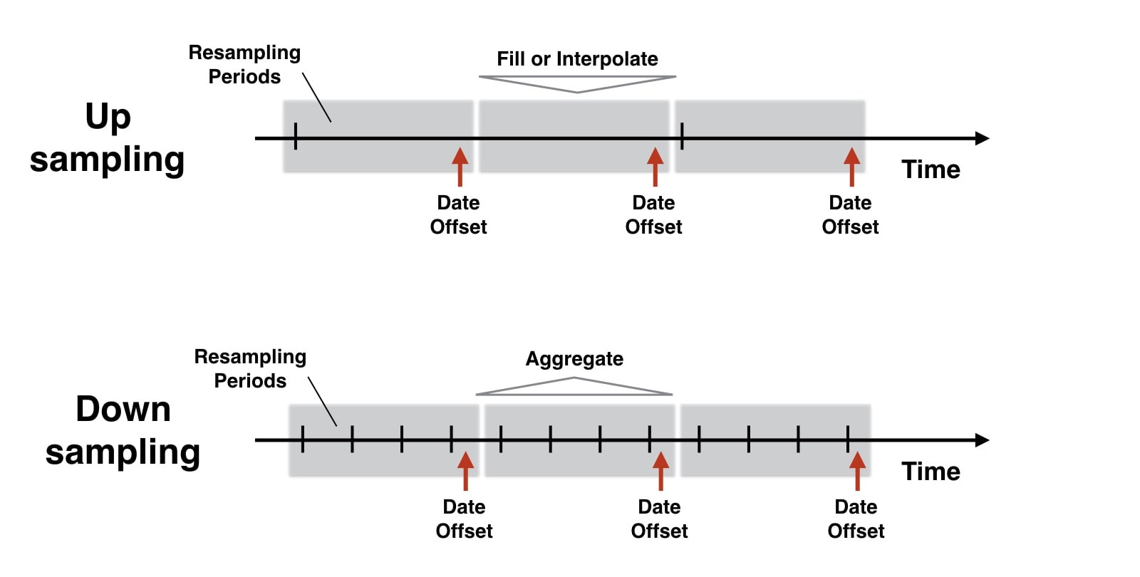
> Types of Resampling
Resampling is generally performed in two ways:
- Upsampling: It happens when you convert time series from lower frequency to higher frequency like from month-based to day-based or hour-based to minute-based.
- When time series data is converted from lower frequency to higher frequency then a number of observations increases hence we need a method to fill newly created frequency.
- Downsampling: It happens when you convert time series from higher frequency to lower frequency like from week-based to month-based, hour-based to day-based, etc.
- When you convert time series from higher frequency to lower frequency then the number of samples will decrease and also it'll result in loss of some values.
1.1 Resampling Data using "asfreq()" Method 
The first method that we'll like to introduce is asfreq() method for resampling. Pandas series, as well as dataframe objects, have this method available which we can call on them.
> Important Parameters of "asfred()" Method
The asfreq() method accepts important parameters like freq, method, and fill_value.
- freq parameter lets us specify a new frequency for time series object.
- method parameter provides a list of methods like ffill, bfill, backfill and pad for filling in newly created indexes when we up-sampled time series data.
- Forward fill will fill newly created indexes with values in previous indexes whereas backward fill will fill the newly created indexes with values from the next index value.
- pad method will fill in with the same values for a particular time interval.
- The default value for method parameter is None and it puts NaNs in newly created indexes when upsampling.
- fill_value lets us fill in NaNs with a value specified as this parameter. It does not fill existing NaNs in data but only NaNs which are generated by asfreq() when resampling data.
We'll now explore the usage of asfreq() below with few examples.
Below, we have created a simple pandas series with datetime index. If you are someone who is new to date_range() function to generate date ranges then please check below link. We have covered how to work with dates, timestamps, time deltas, periods, and time zones in Python using pandas.
rng = pd.date_range(start = "1-1-2020", periods=5, freq="H")
ts = pd.Series(data=range(5), index=rng)
ts
1.1.1 Upsampling Examples
Below we are trying a few examples to demonstrate upsampling. We'll explore various methods to fill in newly created indexes.
ts.asfreq(freq="30min")
We can notice from the above example that asfreq() method by default put NaN in all newly created indexes. We can either pass a value to be filled in into these newly created indexes by setting fill_value parameter or we can call any fill method as well. We'll explain it below with few examples.
ts.asfreq(freq="30min", fill_value=0.0)
We can see that the above example filled in all NaNs with 0.0.
ts.asfreq(freq="30min", method="ffill")
We can notice from the above examples that ffill method filled in a newly created index with the value of previous indexes.
ts.asfreq(freq="45min", method="ffill")
ts.asfreq(freq="45min", method="bfill")
ts.asfreq(freq="45min", method="pad")
df = pd.DataFrame({"TimeSeries":ts})
df
df.asfreq(freq="45min")
df.asfreq(freq="45min", fill_value=0.0)
df.asfreq("30min", method="ffill")
df.asfreq("30min", method="bfill")
df.asfreq("30min", method="pad")
1.1.2 Downsampling
We'll now explain a few examples of downsampling.
ts.asfreq(freq="1H30min")
ts.asfreq(freq="1H30min", fill_value=0.0)
ts.asfreq(freq="1H30min", method="ffill")
ts.asfreq(freq="1H30min", method="bfill")
ts.asfreq(freq="1H30min", method="pad")
df.asfreq(freq="1H30min")
df.asfreq(freq="1H30min", fill_value=0.0)
df.asfreq(freq="1H30min", method="ffill")
df.asfreq(freq="1H30min", method="bfill")
df.asfreq(freq="1H30min", method="pad")
We can lose data sometimes when doing downsampling and the asfreq() method just uses a simple approach to downsampling. It provides only method "bfill", "ffill", and "pad" for filling in data when upsampling or downsampling.
What if we need to apply some other function than these three functions?
We need a more reliable approach to handle resampling. Pandas provide another method called "resample()" which can help us with that.
1.2 Resampling Data using "resample()" Method 
The resample() method accepts new frequency to be applied to time series data and returns "Resampler" object. We can apply various methods other than bfill, ffill and pad for filling in data when doing upsampling / downsampling.
The Resampler object supports a list of aggregation functions like mean, std, var, count, etc which will be applied to time-series data when doing upsampling or downsampling.
We'll now explain the usage of resample() below with few examples.
1.2.1 Downsampling Examples
We are below trying various ways to downsample the data below.
ts.resample("1H30min").mean()
The above example is taking mean of index values appearing in that 1 hour and 30-minute windows. Out time series is sampled at 1 hour so in 1 hour and 30 minutes window generally, 2 values will fall in. It'll take mean of that values when downsampling to the new index. We can call functions other than mean() like std(), var(), sum(), count(),interpolate() etc.
ts.resample("1H15min").mean()
ts.resample("1H15min").std()
ts.resample("1H15min").var()
ts.resample("1H15min").sum()
ts.resample("1H15min").count()
ts.resample("1H15min").bfill()
ts.resample("1H15min").ffill()
1.2.2 Upsampling Examples
We'll now try below a few examples by upsampling time series.
NOTE
Please make a note that we can even apply our own defined function to "Resampler" object by passing it to "apply()" method on it.
ts.resample("45min").bfill()
ts.resample("45min").apply(lambda x: x**2 if x.values.tolist() else np.nan)
ts.resample("45min").interpolate()
df.resample("45min").mean().fillna(0.0)
The above examples clearly state that resample() is a very flexible function and lets us resample time series by applying a variety of functions.
Which One to Use for Resampling Time Series Data? "asfreq()" or "resample()"
Please make a note that in order for "asfreq()" and "resample()" to work, time series data should be sorted according to time else it won't work. It's also suggested to use "resample()" more frequently than "asfreq()" because of its flexibility.
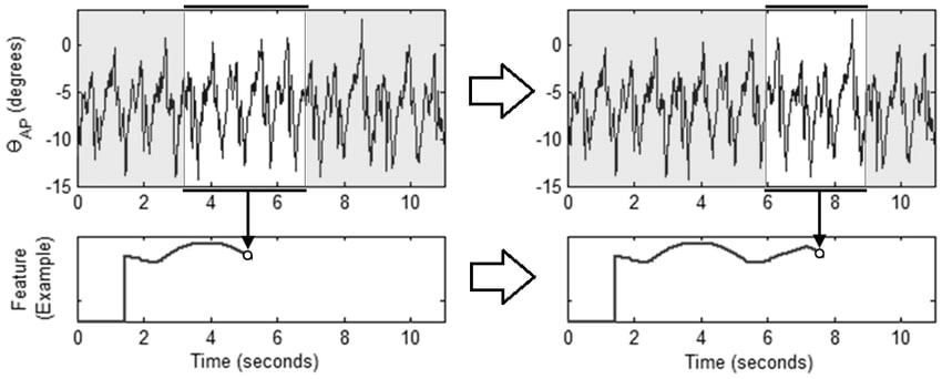
2. How to Apply Moving Window Functions to Time Series Data using Pandas?
Moving window functions refers to functions that can be applied to time-series data by moving fixed / variable size window over total data and computing descriptive statistics over window data each time.
Here window generally refers to a number of samples taken from total time series in order and represents a particular represents period of time.
> Types Of Moving Window Functions
There are 2 kinds of window functions:
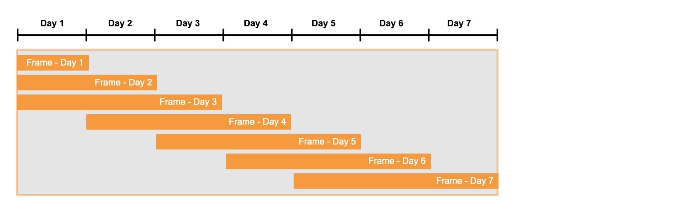
- Rolling Window Functions: It performs aggregate operations on the window with the same amount of sample each time.
- Expanding Window Functions: It performs aggregate operations on the window which expands with time.
> Pandas Methods to Perform Moving Window Operations
Below, we have listed methods Pandas provides for performing window functions. We can call them on series and dataframe both.
- rolling() - Method to perform rolling window operations on time series data available as pandas series or dataframe.
- expanding() - Method to perform expanding window operations on time series data available as pandas series or dataframe.
- ewm() - Method to perform exponential weighted moving average operations on time series data available as pandas series or dataframe.
2.1 Rolling Window Calculations using "rolling()" Method 
The rolling() function lets us perform rolling window functions on time series data.
The rolling() function can be called on both series and dataframe in pandas. It accepts window size as a parameter to group values by that window size and returns Rolling objects which have grouped values according to window size. We can then apply various aggregate functions (mean(), std(), var(), sum(), etc) on this object as per our needs.
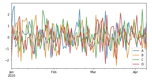
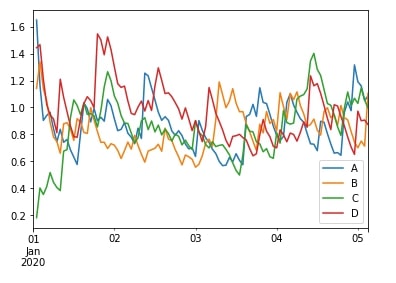
We'll create a simple dataframe of random data to explain this further.
df = pd.DataFrame(np.random.randn(100, 4),
                  index = pd.date_range('1/1/2020', periods = 100),
                  columns = ['A', 'B', 'C', 'D'])

df.head()
df.plot(figsize=(8,4));
r = df.rolling(3)
r
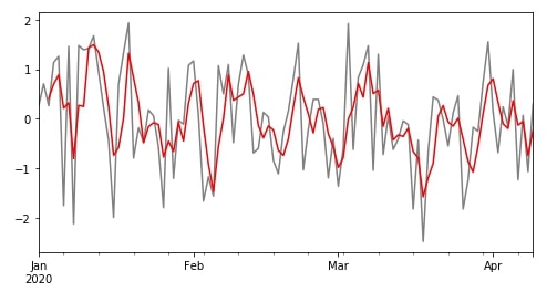
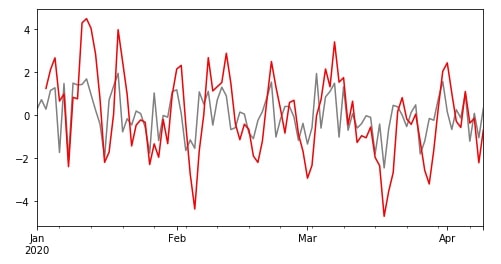
Above, We have created a rolling object with a window size of 3. We can now apply various aggregate functions on this object to get a modified time series. We'll start by applying a mean function to a rolling object and then visualize data of column B from the original dataframe and rolled output.
df["B"].plot(color="grey", figsize=(8,4));
r.mean()["B"].plot(color="red");
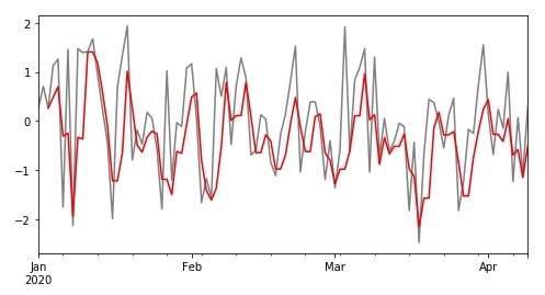
There are many other descriptive statistics functions available which can be applied to rolling object like count(), median(), std(), var(), quantile(), skew(), etc. We can try a few below for our learning purpose.
df["B"].plot(color="grey", figsize=(8,4));
r.quantile(0.25)["B"].plot(color="red");
df["B"].plot(color="grey", figsize=(8,4));
r.skew()["B"].plot(color="red");
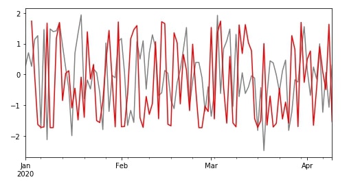
df["B"].plot(color="grey", figsize=(8,4));
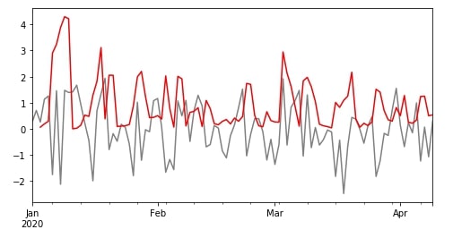
r.var()["B"].plot(color="red");
We can even apply our own function by passing it to apply() function. We are explaining its usage below with an example.
NOTE
Please make a note that input to function passed to "apply()" will be numpy array of samples same as window size.
df["B"].plot(color="grey", figsize=(8,4));
r.apply(lambda x: x.sum())["B"].plot(color="red");
We can apply more than one aggregate function by passing them to agg() function. We'll explain it below with an example. We can apply aggregate functions to only one column as well as ignore other columns.
r.agg(["mean", "std"]).head()
r["A"].agg(["mean", "std"]).head()
We can perform a rolling window function on data samples at a different frequency than the original frequency as well. We'll below load data as hourly and then apply rolling window function by daily sampling that data.
df = pd.DataFrame(np.random.randn(100, 4),
                  index = pd.date_range('1/1/2020', freq="H", periods = 100),
                  columns = ['A', 'B', 'C', 'D'])
df.head()
df.resample("1D").mean().rolling(3).mean().head()
df.resample("1D").mean().rolling(3).mean().plot();
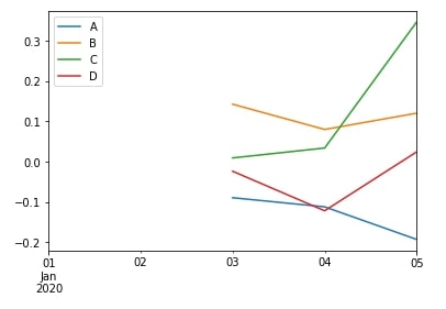
We can notice above that our output is with daily frequency than the hourly frequency of original data.
2.2 Expanding Window Calculations using "expanding()" Method 
Pandas provided a function named expanding() to perform expanding window functions on our time series data.
The expanding() function can be called on both series and dataframe in pandas.
As we discussed above, expanding window functions are applied to total data and take into consideration all previous values, unlike the rolling window which takes fixed-size samples into consideration. We'll explain its usage below with few examples.
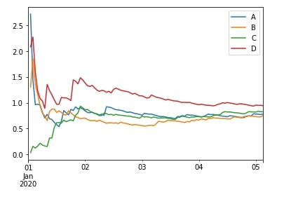
df.expanding(min_periods=1).mean().head()
df.expanding(min_periods=1).mean().plot();
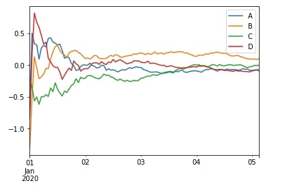
We can notice from the above plot that the output of expanding the window is fluctuating at the beginning but then settling as more samples come into the computation. The output fluctuates a bit initially due to less number of samples taken into consideration initially. The number of samples increases as we move forward with computation and keeps on increasing till the whole time series has been completed.
We can apply various aggregation function to expanding window like count(), median(), std(), var(), quantile(), skew(), etc. We'll explain them below with few examples.
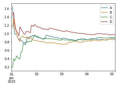
df.expanding(min_periods=1).std().plot();
df.expanding(min_periods=1).var().plot();
We can apply more than one aggregation function by passing their names as a list to agg() function as well as we can apply our own function by passing it to apply() function. We have explained both usages below with examples.
df.expanding(min_periods=1).agg(["mean", "var"]).head()
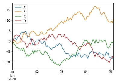
df.expanding(min_periods=1).apply(lambda x: x.sum()).plot();
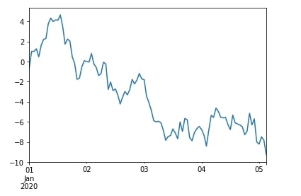
df["A"].expanding(min_periods=1).apply(lambda x: x.sum()).plot();
We'll generally use expanding() windows function when we care about all past samples in time series data even though new samples are added to it. We'll use it when we want to take all previous samples into consideration. We'll use rolling() window functions when only the past few samples are important and all samples before it can be ignored.
2.3 Exponential Weighted Calculations using "ewm()" Method 
An exponential weighted moving average is a weighted moving average of last n samples from time-series data.
The ewm() function can be called on both series and dataframe in pandas.
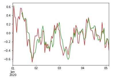
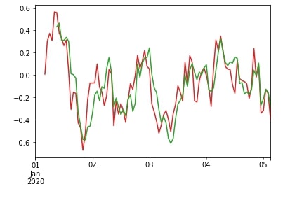
The exponential weighted moving average function assigns weights to each previous sample which decreases with each previous sample. We'll explain its usage by comparing it with rolling() window function.
df["A"].ewm(span=10).mean().plot(color="tab:red");
df["A"].rolling(window=10).mean().plot(color="tab:green");
df["A"].ewm(span=10, min_periods=5).mean().plot(color="tab:red");
df["A"].rolling(window=10).mean().plot(color="tab:green");
We can apply different kinds of aggregation functions as we applied above with rolling() and expanding() functions. We'll try below a few examples for explanation purposes.
df.ewm(span=10).std().plot();
df.ewm(span=10).agg(["mean", "var"]).head()
This concludes our small tutorial on resampling and moving window functions with time-series data using pandas.
References 
- Time-Series : Dates, Times & Time Zone Handling in Python using Pandas
- Time Series Analysis with Python Intermediate | SciPy 2016 Tutorial | Aileen Nielsen
Other Useful Time Series Tutorials
 Sunny Solanki
Sunny Solanki
Intro: Software Developer | Youtuber | Bonsai Enthusiast
About: Sunny Solanki holds a bachelor's degree in Information Technology (2006-2010) from L.D. College of Engineering. Post completion of his graduation, he has 8.5+ years of experience (2011-2019) in the IT Industry (TCS). His IT experience involves working on Python & Java Projects with US/Canada banking clients. Since 2020, he’s primarily concentrating on growing CoderzColumn.
His main areas of interest are AI, Machine Learning, Data Visualization, and Concurrent Programming. He has good hands-on with Python and its ecosystem libraries.
Apart from his tech life, he prefers reading biographies and autobiographies. And yes, he spends his leisure time taking care of his plants and a few pre-Bonsai trees.
Contact: sunny.2309@yahoo.in


![YouTube Subscribe]() Comfortable Learning through Video Tutorials?
Comfortable Learning through Video Tutorials?
If you are more comfortable learning through video tutorials then we would recommend that you subscribe to our YouTube channel.
![Need Help]() Stuck Somewhere? Need Help with Coding? Have Doubts About the Topic/Code?
Stuck Somewhere? Need Help with Coding? Have Doubts About the Topic/Code?
 Stuck Somewhere? Need Help with Coding? Have Doubts About the Topic/Code?
When going through coding examples, it's quite common to have doubts and errors.
If you have doubts about some code examples or are stuck somewhere when trying our code, send us an email at coderzcolumn07@gmail.com. We'll help you or point you in the direction where you can find a solution to your problem.
You can even send us a mail if you are trying something new and need guidance regarding coding. We'll try to respond as soon as possible.
![Share Views]() Want to Share Your Views? Have Any Suggestions?
Want to Share Your Views? Have Any Suggestions?
 Want to Share Your Views? Have Any Suggestions?
If you want to
- provide some suggestions on topic
- share your views
- include some details in tutorial
- suggest some new topics on which we should create tutorials/blogs
 time-series, resampling, moving-window-functions