PyTorch: LSTM Networks for Time-Series Data (Regression Tasks)¶

Time-Series data is measured at a particular interval of time. It has a time component commonly referred to as the temporal component and is represented as time/date/date-time. Time series data can have one (Univariate) or more data variables (Multi-Variate) measured at a specified interval of time. The most common example of time-series data is stock prices measured every minute/hour/day. Time-series data is different from other data used for Machine learning tasks because the order of the data matters and we can not shuffle examples as we do with other ML tasks. When making predictions for an example with time-series data, we generally use the previous few examples. When using neural networks for solving time-series data tasks, Recurrent Neural Networks (RNNs) and their variants have proven to perform quite well. The reason behind this is that RNNs are good at capturing sequences of data and time-series data has sequence that needs to be captured to make proper predictions.

As a part of this tutorial, we have explained how we can create Recurrent Neural Networks (RNNs) that uses LSTM Layers using Python Deep Learning library PyTorch for solving time-series regression tasks. The dataset we have used for our purpose is multi-variate dataset named Tetouan City Power Consumption available from UCI ML Datasets Repository. The dataset has variables temperature, humidity, wind speed, diffuse flows, and power consumption measured every 10 minutes. We'll be predicting power consumption which is a continuous variable hence the task will be considered as regression task.

Below, we have listed essential sections of the Tutorial to give an overview of the material covered.

Important Sections Of Tutorial¶

1. Prepare Data
   • 1.1 Download Data
   • 1.2 Load Data
   • 1.3 Organize Data
   • 1.4 Scale Target Values
   • 1.5 Create Data Loaders
2. Define LSTM Network
3. Train Network
4. Evaluate Network Performance
5. Visualize Predictions on Test Data
6. Further Suggestions

Below, we have imported the necessary Python libraries that we have used in our tutorial and printed the versions of them.

1. Prepare Data ¶

In this section, we are preparing dataset for the task. We have downloaded the dataset from UCI repository and organized it so that it can be processed by the network. As we had said earlier, when making a prediction about a particular example, the best available data is the previous day's data or the previous few days' data. We need to lookback data of the previous few examples to make a prediction of the current as the current day's other data variables won't be available. We have followed the below steps to prepare data for LSTM network.

1. Download data and load it.
2. Move window of pre-decided size (lookback) through data taking that many examples as data features and the next example after them as target value. To explain it with an example,
   • Take data variables from examples 1-30 as lookback (X) of 31st target value (Y).
   • Move the window by one example.
   • Take data variables from examples 2-31 as lookback (X) of 32nd target value (Y).
   • Move the window by one example
   • Take data variables from examples 3-32 as lookback (X) of the 33rd target value (Y).
   • Move the window by one example
   • and so on.
3. Create data loaders using organized datasets.

Though in our example, we are looking at the past few days' data to make predictions of the current, we can make predictions of the next few days as well by looking at the past few days' data. For example, by looking at the last 15 days' data, we can make predictions for the next 5 days. It is not necessary to predict just one day in the future.

Don't worry if the steps are not clear to you in words. They'll become clear as we perform them below.

1.1 Download Data¶

Here we have downloaded our Tetouan City Power Consumption dataset from the UCI ML repository using wget command. It has power consumption information of three different distribution networks of Tetouan city located in the north of morocco.

1.2 Load Data¶

In this section, we have first loaded the dataset into memory using Python library pandas. We have loaded the dataset as a pandas dataframe which is commonly used to load 2d data into memory. After loading the dataset, we converted datetime column data into the proper format and made it an index of our dataframe. The data is measured every 10 minutes as we can see from the first few rows. The dataset has the below columns.

1. Date-time
2. Temperature
3. Humidity
4. Wind Speed
5. General diffuse flows
6. Diffuse flows
7. Zone 1 Power Consumption (units)
8. Zone 2 Power Consumption
9. Zone 3 Power Consumption

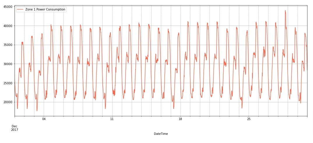
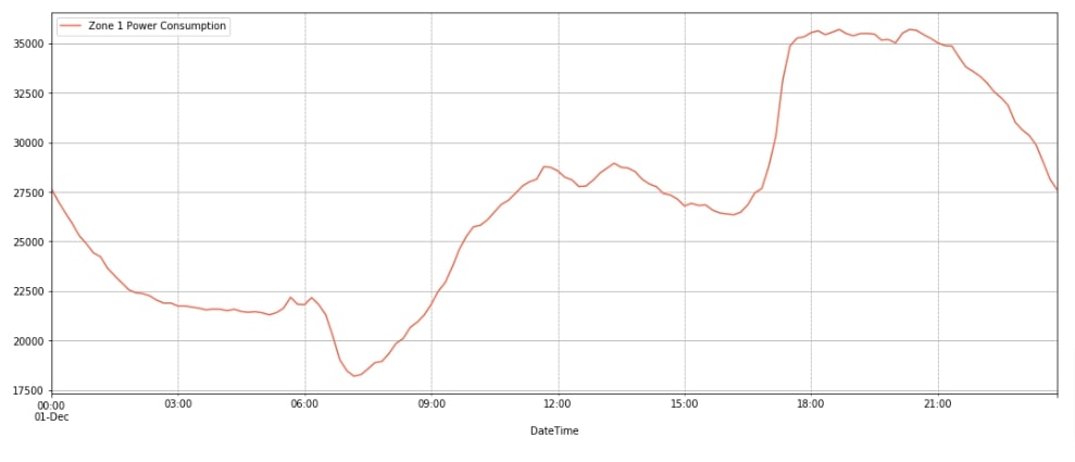
We'll be using columns Temperature, Humidity, Wind Speed, General diffuse flows, and Diffuse flows as data features (independent variables - X). Column Zone 1 Power Consumption will be our target value (dependent variable - Y) that we'll predict. The dataset has entries from 2017-1 till 2017-12. After loading the dataset, we have also plotted power consumption for December 2017 as a line chart. We have also plotted the power consumption for a single day. We can notice from the line charts that power consumption has seasonality (daily) and trend (little increase in consumption over time) as well.

1.3 Organize Data¶

After loading the dataset in memory, in this section, we have organized the dataset. We have decided to use look 30 previous examples to make predictions for the current example. As data is measured every 10 minutes, 30 examples will be the last 5 hours of data. We have set columns ['Temperature', 'Humidity', 'Wind Speed', 'general diffuse flows', 'diffuse flows'] as data features and column Zone 1 Power Consumption as target column. We are then looping through data by moving a window of size 30. For each example, the previous 30 examples' data features will be data features. They will be used to predict the target value of the current example.

After creating data features (X_organized) and target values (Y_organized) arrays, we have divided them into the train (X_train, Y_train) and test sets (X_test, Y_test). We have taken the first 50k examples for training purposes and the remaining 2.3k+ examples for the test dataset. We have also converted datasets to torch tensors as required by PyTorch networks.

1.4 Scale Target Values¶

In this section, we have scaled the values of the target column. The reason behind this is that the values of the target column have high values compared to other columns. This can prevent the optimization algorithm from converging. The values of other data feature columns are generally in the range 0-100. If data features columns had high values then we would have scaled them as well. The scaling helps the optimization algorithm converge faster.

To scale target values, we first calculated the mean and standard deviation of train values. Then, we subtracted the mean from train/test values and divided subtracted values by standard deviation. After scaling values, we have printed new min-max of target values as well. When making a prediction, we'll remove this scaling by reversing these steps.

1.5 Create Data Loaders¶

In this section, we have simply created data loaders which will be used to loop through training data in batches during the training process. We have prevented the shuffle of text examples by setting shuffle to False. We have set batch size to 32.

2. Define LSTM Network ¶

In this section, we have defined a network that we'll use for our time-series regression task. The network consists of three layers, two LSTM layers followed by a dense layer. The lstm layers have output units of 256 and the dense layer has a single output unit. We have created LSTM layers using LSTM() constructor where we have set num_layers parameter to 2 asking it to stack two LSTM layers. The input shape of first LSTM layer is (batch_size, lookback, n_features) = (batch_size, 30, 5) and output shape is (batch_size, 30, 256). The output of the first LSTM layer is given to the second LSTM layer for processing whose output shape is (batch_size, 30, 256). The output of the second LSTM layer is given to a dense layer whose output shape is (batch_size, 1) which is a prediction of our network.

After defining the network, we initialized it and printed the shapes of weights/biases of layers. We have also performed a forward pass-through network using random data for verification purposes.

Please make a NOTE that we have not explained how LSTM layers work internally. Also, We have not covered details of designing networks using PyTorch as we assume that the reader already has little background on them. If you are new to these topics then we recommend that you go through the below tutorials to get background on them.

• PyTorch: Neural Networks using "torch.nn" Module
• PyTorch: LSTM Networks for Text Classification Tasks

3. Train Network ¶

In this section, we are training our network. We have created a simple function that we'll use for training our network. The function takes model, loss function, optimizer, train data loader, validation data loader, and a number of epochs as input. It then executes a training loop number of epochs time. During each epoch, we loop through training data in batches using a train data loader. For each batch of data, we perform a forward pass to make predictions, calculate loss, calculate gradients, and update network parameters (weights & biases). We keep track of loss at each batch and print the average loss of all batches at the end of each epoch. We have also created a helper function that calculates the loss of the model on validation data and prints it.

Below, we are actually training our network by calling the training routines we designed in the previous cell. We have initialized a number of epochs to 20 and the learning rate to 0.001. Then, we have initialized mean squared error loss function, our regression network, and Adam optimizer (to update network parameters). At last, we have called our training routine with the necessary parameters to perform training. We can notice from the loss values getting printed after each epoch that our network is doing a good job because the loss is decreasing constantly.

4. Evaluate Network Performance ¶

In this section, we have evaluated the performance of our trained network on the test dataset. We have made predictions on our test dataset first. After making predictions, we multiplied predictions by standard deviation and added the mean of train data we calculated earlier. This step is done to scale data back to the original range.

Then, we have calculated R2 score and mean squared error metrics on test predictions. The R2 score has values in the range [0,1] and values near 1 are considered sign of good model. From our calculated score, we can confirm that our model is doing a good job at predicting unit consumption. We have calculated these metrics using functions available from scikit-learn.

If you want to understand in-depth how these metrics work internally then we recommend that you go through the below link. Our tutorial covers the majority of ML functions available through sklearn.

• Scikit-learn: Model Evaluation and Scoring Metrics

5. Visualize Predictions on Test Data ¶

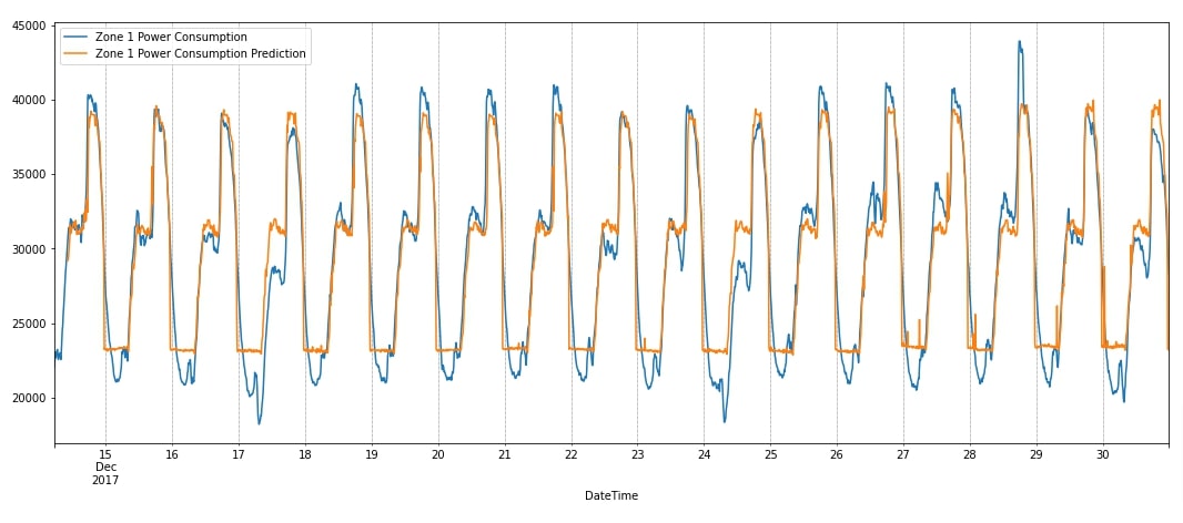
In this section, we have added our predictions to the test dataset and visualized them using matplotlib to show how our network has performed. The chart has original unit consumption as well as predicted consumption for Zone 1. We can notice from the visualization that our network seems to have properly captured seasonality. It even has tried to capture trends in data though it is less visible. It is properly capturing peaks in data but is not able to capture drops that well. In the next section, we have given a few suggestions for improving network performance further.

6. Further Suggestions ¶

• Try different lookback values. We have used 30 previous values to make predictions of the current.
• Make architecture predict more than one target value. We have created an architecture that only predicts one future target value. We can create a network that predicts 5 or 10 future target values as well. The data needs to be organized in that way and the output units of the last dense layer should be the same as our selected number of future target values.
• Try adding features to data from datetime like a weekday, month-end/month-start, month, AM/PM, etc.
• Try different output units for LSTM layers.
• Stack more LSTM layers (This can increase training time).
• Try adding more dense layers after LSTM layers.
• Try different weight initialization methods.
• Try learning rate schedulers

References¶

• Time-Series: Re-sampling and Moving Window Functions
• Guide to Remove Trend and Seasonality from Time-Series Data
• Date, Time and Time-Zone Handling in Python (Pandas)
• Python Module: time
• Python Module: datetime