Simple Guide to Learning Rate Schedules for Keras Networks
When training Python Keras networks using optimizers like stochastic gradient descent (SGD), the learning rate of the network stays constant throughout the training process. This will work in many scenarios. But as we get closer to optima, reducing a learning rate a bit over time can help get better results. It can boost the performance of the model. There are various ways to reduce the learning rate over time during the training process. It's commonly referred to as learning rate scheduling or learning rate annealing. Keras provides many learning rate schedulers that we can use to anneal the learning rate over time.
As a part of this tutorial, we'll discuss various learning rate schedulers available from keras as well as, we'll explain how one can implement a custom scheduler if existing schedulers do not satisfy their requirements. We have used the Fashion MNIST dataset for our tutorial and have trained a simple convolutional neural network on it to explain various schedulers.
Below, we have highlighted important sections of tutorial to give an overview of the material covered.
Important Sections Of Tutorial
- Load Fashion MNIST Dataset
- Define CNN Model
- Train Network With Different Schedulers
Below, we have loaded keras and printed the version of it that we'll use in our tutorial.
import tensorflow as tf
from tensorflow import keras

print("Keras Version : {}".format(keras.__version__))
Load Fashion MNIST Dataset 
In this section, we have loaded the Fashion MNIST dataset available from the keras detasets module. The dataset has grayscale images of size (28,28) pixels for 10 different fashion items. The dataset is already divided into the train (60k images) and test (10k images) sets. The below table shows the mapping from index to fashion item names.
| Label | Description |
|---|---|
| 0 | T-shirt/top |
| 1 | Trouser |
| 2 | Pullover |
| 3 | Dress |
| 4 | Coat |
| 5 | Sandal |
| 6 | Shirt |
| 7 | Sneaker |
| 8 | Bag |
| 9 | Ankle boot |
from tensorflow.keras import datasets
import numpy as np
from tensorflow.keras.utils import to_categorical

(X_train, Y_train), (X_test, Y_test) = datasets.fashion_mnist.load_data()

X_train,X_test = X_train.reshape(-1,28,28,1), X_test.reshape(-1,28,28,1)
Y_train, Y_test = to_categorical(Y_train), to_categorical(Y_test)

classes =  np.unique(Y_train)

X_train.shape, X_test.shape, Y_train.shape, Y_test.shape
Define CNN Model 
In this section, we have defined the CNN that we'll be using for our classification task when explaining various learning rate schedules. We have created a simple function that will create a neural network and return it each time it is called. The neural network has the simple architecture of 2 convolution layers followed by one dense layer. The convolution layers have filters of sizes 32 and 16 respectively. Both convolution layers will apply kernels of shape (3,3) on input image data. We have applied relu (rectified linear unit) activation after each convolution layer application. Then, we have flattened the output of the second convolution layer and has filled it into a dense layer that has 10 output units (same as a number of classes). The output of the dense layer has been converted to probabilities by applying softmax activation function.
from tensorflow.keras import Sequential
from tensorflow.keras import layers

def create_model():
    return Sequential([
                    layers.Conv2D(filters=32, kernel_size=(3,3), padding="same", activation="relu", input_shape=(28,28,1)),
                    layers.Conv2D(filters=16, kernel_size=(3,3), padding="same", activation="relu"),

                    layers.Flatten(),
                    layers.Dense(10, activation="softmax")
                    ])

model = create_model()
model.summary()
1. Constant Learning Rate With SGD 
In this section, we have trained our CNN using SGD which has a constant learning rate. We have set the learning rate to a constant value of 0.001. We have trained the network for only 5 epochs.
from tensorflow.keras.optimizers import SGD

grad_descent = keras.optimizers.SGD(learning_rate=0.001)

model.compile(optimizer=grad_descent, loss="categorical_crossentropy", metrics=["accuracy"])

model.fit(x=X_train, y=Y_train, batch_size=64, epochs=5, validation_data=(X_test,Y_test))
2. SGD With Decay 
In this section, we are training the neural network again with SGB but this time we have provided decay rate as well. It'll decay the learning rate by following the below formula.
learning_rate = learning_rate / (1. + decay * local_step)
In the next cell after training, we have also printed the code that has logic to handle decay in the keras codebase. We have used the python inspect module for retrieving code.
model = create_model() ##

epochs = 5
lr = 0.001

grad_descent = keras.optimizers.SGD(learning_rate=lr, decay=lr/epochs)

model.compile(optimizer=grad_descent, loss="categorical_crossentropy", metrics=["accuracy"])

model.fit(x=X_train, y=Y_train, batch_size=64, epochs=epochs, validation_data=(X_test,Y_test))
import inspect

print("====== SGD Source ====================================")
print(inspect.getsource(keras.optimizers.SGD)[:510])
print()
print("====== Decay Learning Rate Method ====================")
print(inspect.getsource(keras.optimizers.Optimizer._decayed_lr))
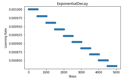
3. Exponential Decay 
In this section, we have trained our network using SGD with exponential decay. We can create an instance of exponential decay using ExponentialDecay constructor available from keras.optimizers.schedules module. It has the below-mentioned important parameters.
- initial_learning_rate - This parameter accepts the initial learning rate of the optimizer.
- decay_steps - Number of steps after which to reduce learning rate. Here, one step refers to the execution of one batch of data.
- decay_rate - The float value specifying decay rate.
- staircase - This parameter accepts boolean value which if set to True will follow staircase function.
The decayed learning rate is calculated using the below formula.
learning_rate = initial_learning_rate * decay_rate ^ (step / decay_steps)
Below, we have created an exponential decay with an initial learning rate of 0.001, 500 decay steps, and a decay rate of 0.98. This scheduler will decay the learning rate after every 500 steps/batches. We have provided a scheduler to SGD.
In the next cell after the training cell, we have also retrieved the learning rate for 5000 steps and plotted them to give an idea of how the learning rate will change during our training process. In our case, the dataset has 60k images and we have used 64 samples per batch which will bring a number of steps per epoch to ~1000. As we are training for 5 epochs, the total steps will be ~5000.
from tensorflow.keras.optimizers.schedules import ExponentialDecay

model = create_model()  ## Create Model

epochs = 5
lr = 0.001

lr_schedule = ExponentialDecay(lr, decay_steps=500, decay_rate=0.98, staircase=True)

grad_descent = keras.optimizers.SGD(learning_rate=lr_schedule)

model.compile(optimizer=grad_descent, loss="categorical_crossentropy", metrics=["accuracy"])

model.fit(x=X_train, y=Y_train, batch_size=64, epochs=epochs, validation_data=(X_test,Y_test))
import matplotlib.pyplot as plt

lrs = [lr_schedule(step) for step in range(5000)]

plt.scatter(range(5000), lrs);
plt.title("ExponentialDecay");
plt.xlabel("Steps")
plt.ylabel("Learning Rate");
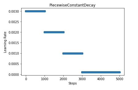
4. Piecewise Constant Decay 
In this section, we are training our network using SGD with a piecewise constant decay scheduler. We can create an instance of piece-wise constant decay scheduler using PiecewiseConstantDecay() constructor available from keras.optimizers.schedules module. It has the below-mentioned parameters.
- boundaries - List of integers specifying boundaries for which learning rate will be constant. This parameter will divide the training process based on a number of steps provided in it and will use the learning rate according to values parameter. It'll become clear when we explain it below with an example.
- values - List of learning rate values for boundaries specified using boundaries parameter. It'll have one value more than boundaries.
In our case, we have set boundaries to [1000,2000,3000] and values to [0.003,0.002,0.001,0.0001]. We know that our training process has ~5000 steps as we explained earlier. This assign learning rate of 0.003 to first 1000 steps, learning rate of 0.002 to steps from 1000 to 2000, learning rate of 0.001 to steps from 2000 to 3000 and learning rate of 0.0001 to steps beyond 3000.
Later on, in the next cell, we have also displayed a plot showing how the learning rate will change during our training of ~5000 steps.
from tensorflow.keras.optimizers.schedules import PiecewiseConstantDecay

model = create_model()  ## Create Model

epochs = 5

lr_schedule = PiecewiseConstantDecay(boundaries=[1000, 2000, 3000], values=[0.003,0.002,0.001, 0.0001])

grad_descent = keras.optimizers.SGD(learning_rate=lr_schedule)

model.compile(optimizer=grad_descent, loss="categorical_crossentropy", metrics=["accuracy"])

model.fit(x=X_train, y=Y_train, batch_size=64, epochs=epochs, validation_data=(X_test,Y_test))
import matplotlib.pyplot as plt

lrs = [lr_schedule(step) for step in range(5000)]

plt.scatter(range(5000), lrs);
plt.title("PiecewiseConstantDecay");
plt.xlabel("Steps")
plt.ylabel("Learning Rate");
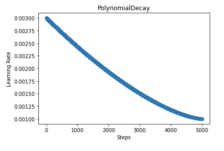
5. Polynomial Decay 
In this section, we have trained our network using SGD with polynomial decay. We can create an instance of polynomial decay using PolynomialDecay() constructor available from keras.optimizers.schedules module. It has the below-mentioned parameters.
- initial_learning_rate - This is the initial learning rate of the training.
- decay_steps - Total number of steps for which to decay learning rate.
- end_learning_rate - Final learning rate below which learning rate should not go.
- power - Float to calculate decay learning rate. If we provide a value less than 1 then the curve of learning rate will be concave else it'll be convex (see below plot).
It uses the below formula to calculate the learning rate at any step.
def decayed_learning_rate(step):
  step = min(step, decay_steps)
  return ((initial_learning_rate - end_learning_rate) *
          (1 - step / decay_steps) ^ (power)
         ) + end_learning_rate
In our case, we have used an initial learning rate of 0.005, an end learning rate of 0.001, and a power value of 1.5.
from tensorflow.keras.optimizers.schedules import PolynomialDecay

model = create_model()  ## Create Model

epochs = 5

lr_schedule = PolynomialDecay(0.003, 5000,0.001, power=1.5)

grad_descent = keras.optimizers.SGD(learning_rate=lr_schedule)

model.compile(optimizer=grad_descent, loss="categorical_crossentropy", metrics=["accuracy"])

model.fit(x=X_train, y=Y_train, batch_size=64, epochs=epochs, validation_data=(X_test,Y_test))
import matplotlib.pyplot as plt

lrs = [lr_schedule(step) for step in range(5000)]

plt.scatter(range(5000), lrs);
plt.title("PolynomialDecay");
plt.xlabel("Steps")
plt.ylabel("Learning Rate");
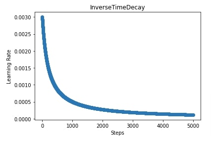
6. Inverse Time Decay 
In this section, we are training our network using SGD with an inverse time decay scheduler. We can create an instance of inverse time decay scheduler using InverseTimeDecay() constructor available from keras.optimizers.schedules module. It has the below-mentioned important parameters.
- initial_learning_rate
- decay_steps - It's an integer specifying number of steps after which decay learning rate.
- decay_rate - It's a float value specifying decay rate.
- staircase
The below formula is used to calculate the learning rate at any step.
def decayed_learning_rate(step):
    return initial_learning_rate / (1 + decay_rate * step / decay_step)
We have created an inverse decay scheduler with an initial learning rate of 0.003, decay steps of 100, and decay rate of 0.5. We have also plotted how the learning rate will change during the training process in the next cell.
from tensorflow.keras.optimizers.schedules import InverseTimeDecay

model = create_model()  ## Create Model

epochs = 5

lr_schedule = InverseTimeDecay(0.003, 100, 0.5)

grad_descent = keras.optimizers.SGD(learning_rate=lr_schedule)

model.compile(optimizer=grad_descent, loss="categorical_crossentropy", metrics=["accuracy"])

model.fit(x=X_train, y=Y_train, batch_size=64, epochs=epochs, validation_data=(X_test,Y_test))
import matplotlib.pyplot as plt

lrs = [lr_schedule(step) for step in range(5000)]

plt.scatter(range(5000), lrs);
plt.title("InverseTimeDecay");
plt.xlabel("Steps")
plt.ylabel("Learning Rate");
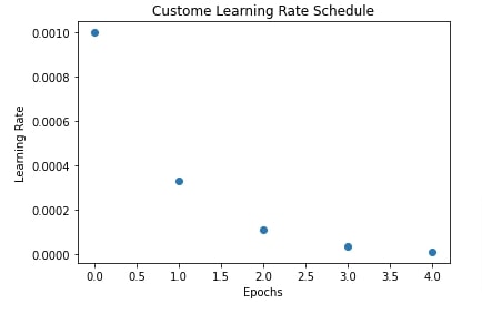
7. Custom Learning Rate Scheduler 
In this section, we have explained how we can create a learning rate scheduler of our own. In order to create a learning rate scheduler, we need to create a function that takes as input epoch number and current learning rate and then returns a new learning rate. Then, we need to wrap this function inside of LearningRateScheduler callback available from keras.callbacks module. We can provide this callback to fit() method and it'll change the learning rate using this function after each epoch. Please make a NOTE that this will change the learning rate after the complete epoch and not for individual steps.
If you want to know about callbacks in keras then please feel free to check the below link.
We have also plotted in the next cell how the learning rate will change over time after each epoch.
def custome_lr_scheduler(epoch, current_lr):
    return current_lr / 3
from keras.callbacks import LearningRateScheduler
from tensorflow.keras.optimizers.schedules import InverseTimeDecay

model = create_model()  ## Create Model

epochs = 5

lr_schedule = LearningRateScheduler(custome_lr_scheduler)

grad_descent = keras.optimizers.SGD(learning_rate=0.001)

model.compile(optimizer=grad_descent, loss="categorical_crossentropy", metrics=["accuracy"])

model.fit(x=X_train, y=Y_train, batch_size=64, epochs=epochs, validation_data=(X_test,Y_test), callbacks=[lr_schedule])
import matplotlib.pyplot as plt

current_lr = 0.001
lrs = [current_lr]

for epoch in range(1,5):
    current_lr = custome_lr_scheduler(epoch, current_lr)
    lrs.append(current_lr)

plt.scatter(range(5), lrs);
plt.title("Custome Learning Rate Schedule");
plt.xlabel("Epochs")
plt.ylabel("Learning Rate");
This ends our small tutorial explaining how we can use learning rate schedulers available from keras to anneal learning rate during the training process. We also explained how we can create our own custom callback. Please feel free to let us know your views in the comments section.
References
 Sunny Solanki
Sunny Solanki
Intro: Software Developer | Youtuber | Bonsai Enthusiast
About: Sunny Solanki holds a bachelor's degree in Information Technology (2006-2010) from L.D. College of Engineering. Post completion of his graduation, he has 8.5+ years of experience (2011-2019) in the IT Industry (TCS). His IT experience involves working on Python & Java Projects with US/Canada banking clients. Since 2020, he’s primarily concentrating on growing CoderzColumn.
His main areas of interest are AI, Machine Learning, Data Visualization, and Concurrent Programming. He has good hands-on with Python and its ecosystem libraries.
Apart from his tech life, he prefers reading biographies and autobiographies. And yes, he spends his leisure time taking care of his plants and a few pre-Bonsai trees.
Contact: sunny.2309@yahoo.in


![YouTube Subscribe]() Comfortable Learning through Video Tutorials?
Comfortable Learning through Video Tutorials?
If you are more comfortable learning through video tutorials then we would recommend that you subscribe to our YouTube channel.
![Need Help]() Stuck Somewhere? Need Help with Coding? Have Doubts About the Topic/Code?
Stuck Somewhere? Need Help with Coding? Have Doubts About the Topic/Code?
 Stuck Somewhere? Need Help with Coding? Have Doubts About the Topic/Code?
When going through coding examples, it's quite common to have doubts and errors.
If you have doubts about some code examples or are stuck somewhere when trying our code, send us an email at coderzcolumn07@gmail.com. We'll help you or point you in the direction where you can find a solution to your problem.
You can even send us a mail if you are trying something new and need guidance regarding coding. We'll try to respond as soon as possible.
![Share Views]() Want to Share Your Views? Have Any Suggestions?
Want to Share Your Views? Have Any Suggestions?
 Want to Share Your Views? Have Any Suggestions?
If you want to
- provide some suggestions on topic
- share your views
- include some details in tutorial
- suggest some new topics on which we should create tutorials/blogs
 learning-rate-schedules, keras