PyTorch RNN For Text Classification Tasks
Neural network types like fully connected networks or convolutional neural networks are good at identifying patterns in data but they do not have a memory. They treat each example of data and parts of the example as independent of each other. They can not maintain any state/memory about previously seen examples. This kind of behavior is good as long as each example like images is independent of each other. But there are situations where remembering state information about previously seen examples can help get better results. Let's say for the natural language processing task of text generation, if our network can remember some state information about words seen, then it can help it remember state and generate new better words as it now knows about the context of the sentence. This kind of approach can help with time-series data as well where new prediction is generally dependent on the last few text examples.
To solve the problem of maintaining memory, Recurrent neural networks (RNN) were introduced. Recurrent neural networks maintain the state of the data examples and use it to improve results. If the reader is interested in learning about the inner workings of RNNs then we recommend this blog which covers it in detail.
As a part of this tutorial, we are going to design simple RNNs using PyTorch to solve text classification tasks. We'll try different approaches to using RNNs to classify text documents. We'll be using the word embedding approach to vectorize words to real-valued vectors before giving them to RNNs. The main aim of the tutorial is to get individuals started using RNNs for text classification tasks. Please check the link below if you are looking for guidance on LSTM Networks (Long Short-Term Memory - a variant of RNNs). It has almost the same structure as this tutorial but explains how to use LSTM networks.
Below, we have listed important sections of tutorial to give an overview of the material covered.
Important Sections Of Tutorial
- Populate Vocabulary
- 1.1 Load Dataset
- 1.2 Create Tokenizer And Populate Vocabulary
- Approach 1: Single RNN Layer (Tokens Per Text Example=25, Embeddings Length=50)
- Load Datasets And Create Data Loaders
- Define RNN Classification Network
- Train Network
- Evaluate Network Performance
- Explain Network Predictions Using LIME Algorithm
- Approach 2: Single RNN Layer (Tokens Per Text Example=50, Embeddings Length=50)
- Approach 3: Multiple RNN Layers (Tokens Per Text Example=50, Embeddings Length=50)
- Approach 4: Stacking Multiple RNN Layers (Tokens Per Text Example=50, Embeddings Length=50)
- Approach 5: Multiple Bidirectional RNN Layers (Tokens Per Text Example=50, Embeddings Length=50)
- Summary of Results And Suggestions
First, we have imported the necessary libraries and printed the versions that we'll use in our tutorial.
import torch

print("PyTorch Version : {}".format(torch.__version__))
import torchtext

print("TorchText Version : {}".format(torchtext.__version__))
1. Populate Vocabulary 
In this section, we have loaded AG NEWS dataset and populated a vocabulary using tokens generated from text examples of the dataset. The vocabulary will then be used to later map tokens to indexes which will be used to identify them. These indexes generated for tokens of text examples will be given as input to neural networks for classifying text documents.
1.1 Load Dataset
In this section, we have simply loaded AG NEWS dataset available from datasets sub-module of torchtext library. The dataset is already divided into the train (120000 text examples) and test (7600 text examples) sets.
from torch.utils.data import DataLoader

train_dataset, test_dataset  = torchtext.datasets.AG_NEWS()
1.2 Create Tokenizer And Populate Vocabulary
In this section, we have populated vocabulary for vectorizing text data using datasets loaded from the previous cell. We have first defined a simple tokenizer using get_tokenizer() function available from data sub-module of torchtext library. The tokenizer is a function that takes a text example as input and returns a list of tokens of that text example. The tokens are general words of the text but they can also be punctuation marks and special symbols.
After defining tokenizer, we have created a vocabulary using build_vocab_from_iterator() function available from vocab sub-module of torchtext library. The function takes an iterator as input that returns a list of tokens on each call. We have created a simple iterator function named build_vocabulary() which takes datasets as input. It then loops through each dataset and text examples from each dataset, yielding a list of tokens for each text example using a tokenizer. The special character <UNK> will be kept at the 0th index and all tokens not present in the dictionary will be mapped to this token.
In the next cells after the below cell, we have printed the length of vocabulary and explained how we can convert text examples to a list of indexes using tokenizer and vocabulary. This list of integers (indexes of tokens/words as per vocabulary) will be given as input to the neural network which will generate embeddings for them.
from torchtext.data import get_tokenizer
from torchtext.vocab import build_vocab_from_iterator

tokenizer = get_tokenizer("basic_english")

def build_vocabulary(datasets):
    for dataset in datasets:
        for _, text in dataset:
            yield tokenizer(text)

vocab = build_vocab_from_iterator(build_vocabulary([train_dataset, test_dataset]), min_freq=1, specials=["<UNK>"])

vocab.set_default_index(vocab["<UNK>"])
len(vocab)
tokens = tokenizer("Hello how are you?, Welcome to CoderzColumn!!")
indexes = vocab(tokens)

tokens, indexes
vocab["<UNK>"] ## Coderzcolumn word is mapped to unknown as it's new and not present in vocabulary
Approach 1: Single RNN Layer (Tokens Per Text Example=25, Embeddings Length=50) 
This is our first approach to the Recurrent layer in our network to classify text documents. We'll be using a combination of embedding, and recurrent and dense layers to create a neural network for classifying text documents. Our network in this approach uses a simple one recurrent neural layer.
Load Datasets And Create Data Loaders
Below, we have loaded AG NEWS dataset again and created data loaders from it that will be used during training to loop through data in batches. We have created train and test data loaders that return a batch of 1024 examples and their respective target labels for each call. We have created a simple vectorization function (vectorize_batch()) that will be used to vectorize text examples of a batch of data. For each batch, it'll tokenize text examples using a tokenizer, generates indexes using vocabulary, and return indexes as torch tensors along with target labels. We have set the maximum token size to 25 which keeps 25 tokens per text example. For examples with more than 25 tokens, extra tokens will be truncated and for examples with less than 25 tokens, they will be padded with 0s (<UNK> token). The function also subtracts 1 from target labels because labels are in the range 1-4 in data and we want them in the range 0-3 for our convenience. The vectorization function is given to collate_fn parameters of both data loaders.
from torch.utils.data import DataLoader
from torchtext.data.functional import to_map_style_dataset

train_dataset, test_dataset  = torchtext.datasets.AG_NEWS()
train_dataset, test_dataset  = to_map_style_dataset(train_dataset), to_map_style_dataset(test_dataset)

target_classes = ["World", "Sports", "Business", "Sci/Tech"]

max_words = 25

def vectorize_batch(batch):
    Y, X = list(zip(*batch))
    X = [vocab(tokenizer(text)) for text in X]
    X = [tokens+([0]* (max_words-len(tokens))) if len(tokens)<max_words else tokens[:max_words] for tokens in X] ## Bringing all samples to max_words length.

    return torch.tensor(X, dtype=torch.int32), torch.tensor(Y) - 1 ## We have deducted 1 from target names to get them in range [0,1,2,3] from [1,2,3,4]


train_loader = DataLoader(train_dataset, batch_size=1024, collate_fn=vectorize_batch, shuffle=True)
test_loader  = DataLoader(test_dataset , batch_size=1024, collate_fn=vectorize_batch)
for X, Y in train_loader:
    print(X.shape, Y.shape)
    break
Define RNN Classification Network
In this section, we have created a neural network that we'll be using for the text classification task. The network consists of 3 layers.
- Embeddings layer
- RNN layer
- Linear layer
The embedding layer has word embeddings for each token/word of our dictionary. We have set an embedding length of 50 for our example. This means that the embedding layer will have the weight of shape (len_vocab, 50). It has an embedding vector of length 50 for each token of our vocabulary. The embedding layer simply maps input indexes to a list of embeddings. Our data loaders will be returning indexes for tokens of text examples which will be given to the embedding layer as input which will convert indexes to embeddings. These embeddings will be updated during training to better classify documents. The input of the embedding layer will be of shape (batch_size, 25) and the output will be (batch_size, 25, 50), The batch size in our case is 1024. If the reader does not have a background on word embeddings then we recommend reading the below article that covers it in detail.
The RNN layer will take input from embedding layer of shape (batch_size, max_tokens, embedding_length) = (batch_size, 25, 50), perform it's operations and return an output of shape (batch_size, max_tokens, hidden_size) = (batch_size, 25, 50). In our case, the output shape of RNN layer is 50. If for example the hidden size of a recurrent layer is set at 75 then output from the recurrent layer will be of shape (batch_size, 25, 75). The recurrent layer loops through embeddings of tokens for each text example and generates output that has some knowledge about the context of the text documents. When calling the recurrent layer in the forward pass, we need to provide initial state detail to it which we have provided as random numbers. An initial state is needed for each text example. If we don't provide it then PyTorch generates a tensor of zeros internally. In our case, we have provided random numbers of shape (1, batch_size, 50) which means for each text example we have provided a real-valued vector of length 50 as an initial state. We recommend that the reader goes through this link if he/she wants to know how RNN layer works internally. Basically, it takes embedding for a single token and the initial state as input and returns the output. This output will become the state for the next token for the text example. For the next token, it'll again take embedding & state (previous output) and returns the new output (state). This process goes till the last token of the text example. This loop is repeated for each text example (25 tokens).
We can create recurrent layer using RNN() constructor available from 'nn' sub-module of torch library. We need to provide input shape and hidden dimension size to the constructor. We can create multiple RNN layers by providing an integer value greater than 1 to num_layers parameter. By default, the output shape of RNN layer will be (25, batch_size, 50) but we have converted it to (batch_size, 25, 50) by setting batch_first parameter to True.
The output of RNN will be given to the linear layer which has 4 output units (same as a number of target classes). We have given the last output of each example (output[:,-1]) in our case to the linear layer because the RNN layer generates output for each 25 tokens of the text example. We only need to give the last output of each example to be given as input to the linear layer as according to the concept of RNN, it has information about all previous tokens. So, even though the output of RNN layer is of shape (batch_size, 25, 50), the input to the linear layer will be (batch_size, 50) because we'll take the last entry from 25 entries for each example.
Please feel free to check the below tutorial if you are new to PyTorch and want to learn how to design networks using it. It's a simple guide for getting started with PyTorch.
After defining the network, we initialized it, printed the shape of weights/biases of layers, and performed a forward pass to make predictions as well. These steps were done for verification purposes that the network works as expected.
from torch import nn
from torch.nn import functional as F

embed_len = 50
hidden_dim = 50
n_layers=1

class RNNClassifier(nn.Module):
    def __init__(self):
        super(RNNClassifier, self).__init__()
        self.embedding_layer = nn.Embedding(num_embeddings=len(vocab), embedding_dim=embed_len)
        self.rnn = nn.RNN(input_size=embed_len, hidden_size=hidden_dim, num_layers=n_layers, batch_first=True)
        self.linear = nn.Linear(hidden_dim, len(target_classes))

    def forward(self, X_batch):
        embeddings = self.embedding_layer(X_batch)
        output, hidden = self.rnn(embeddings, torch.randn(n_layers, len(X_batch), hidden_dim))
        return self.linear(output[:,-1])
rnn_classifier = RNNClassifier()

rnn_classifier
for layer in rnn_classifier.children():
    print("Layer : {}".format(layer))
    print("Parameters : ")
    for param in layer.parameters():
        print(param.shape)
    print()
out = rnn_classifier(torch.randint(0, len(vocab), (1024, max_words)))

out.shape
Train Network
In this section, we are training our network using data loaders. We have created a helper function for the training network. The function takes model, loss function, optimizer, train data loader, validation data loader, and a number of epochs as input. It then performs a training loop number of epochs times. For each epoch, it loops through training data in batches using a train data loader. For each batch of data, it performs a forward pass to make predictions, calculates loss value (using predictions and actual target labels), calculates gradients, and updates network parameters using gradients. It also records the loss value for each batch and prints the average loss at the end of each epoch. We have also created another helper function that loops through the validation data loader and calculates validation accuracy and loss.
from tqdm import tqdm
from sklearn.metrics import accuracy_score
import gc

def CalcValLossAndAccuracy(model, loss_fn, val_loader):
    with torch.no_grad():
        Y_shuffled, Y_preds, losses = [],[],[]
        for X, Y in val_loader:
            preds = model(X)
            loss = loss_fn(preds, Y)
            losses.append(loss.item())

            Y_shuffled.append(Y)
            Y_preds.append(preds.argmax(dim=-1))

        Y_shuffled = torch.cat(Y_shuffled)
        Y_preds = torch.cat(Y_preds)

        print("Valid Loss : {:.3f}".format(torch.tensor(losses).mean()))
        print("Valid Acc  : {:.3f}".format(accuracy_score(Y_shuffled.detach().numpy(), Y_preds.detach().numpy())))


def TrainModel(model, loss_fn, optimizer, train_loader, val_loader, epochs=10):
    for i in range(1, epochs+1):
        losses = []
        for X, Y in tqdm(train_loader):
            Y_preds = model(X)

            loss = loss_fn(Y_preds, Y)
            losses.append(loss.item())

            optimizer.zero_grad()
            loss.backward()
            optimizer.step()

        print("Train Loss : {:.3f}".format(torch.tensor(losses).mean()))
        CalcValLossAndAccuracy(model, loss_fn, val_loader)
Below, we have initialized the necessary parameters and trained our network using a function defined in the previous cell. We have initialized a number of epochs to 15 and the learning rate to 0.001. Then, we have initialized the loss function, our classification network, and Adam optimizer. At last, we have called our training routine with the necessary parameters to perform training. We can notice from the loss and accuracy value getting printed after each epoch that our model is doing a good job at the text classification task.
from torch.optim import Adam

epochs = 15
learning_rate = 1e-3

loss_fn = nn.CrossEntropyLoss()
rnn_classifier = RNNClassifier()
optimizer = Adam(rnn_classifier.parameters(), lr=learning_rate)

TrainModel(rnn_classifier, loss_fn, optimizer, train_loader, test_loader, epochs)
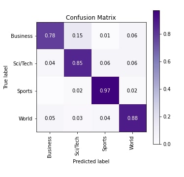
Evaluate Network Performance
In this section, we have evaluated the performance of our network by calculating accuracy, classification report (precision, recall, and f1-score per target class) and confusion matrix metrics on test predictions. We can notice from the accuracy that our model has done a decent job at classifying text documents of the test dataset.
We have used metrics available from scikit-learn to calculate our metrics. Please feel free to check the below link if you want to learn about various metrics available from sklearn.
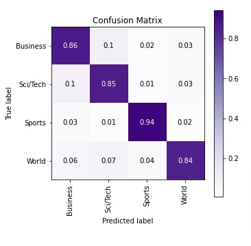
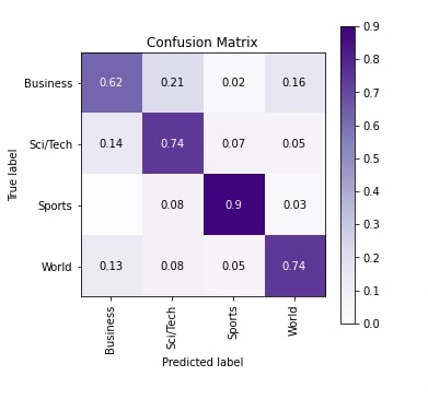
In the next cell after metrics calculation, we have plotted the confusion matrix using scikit-plot python library. We can notice from the visualization that our model is doing a good job at identifying Sports category documents compared to other categories.
If you are interested in learning about scikit-plot which provides visualizations for many ML metrics then please check the below link.
def MakePredictions(model, loader):
    Y_shuffled, Y_preds = [], []
    for X, Y in loader:
        preds = model(X)
        Y_preds.append(preds)
        Y_shuffled.append(Y)
    gc.collect()
    Y_preds, Y_shuffled = torch.cat(Y_preds), torch.cat(Y_shuffled)

    return Y_shuffled.detach().numpy(), F.softmax(Y_preds, dim=-1).argmax(dim=-1).detach().numpy()

Y_actual, Y_preds = MakePredictions(rnn_classifier, test_loader)
from sklearn.metrics import accuracy_score, classification_report, confusion_matrix

print("Test Accuracy : {}".format(accuracy_score(Y_actual, Y_preds)))
print("\nClassification Report : ")
print(classification_report(Y_actual, Y_preds, target_names=target_classes))
print("\nConfusion Matrix : ")
print(confusion_matrix(Y_actual, Y_preds))
from sklearn.metrics import confusion_matrix
import scikitplot as skplt
import matplotlib.pyplot as plt
import numpy as np

skplt.metrics.plot_confusion_matrix([target_classes[i] for i in Y_actual], [target_classes[i] for i in Y_preds],
                                    normalize=True,
                                    title="Confusion Matrix",
                                    cmap="Purples",
                                    hide_zeros=True,
                                    figsize=(5,5)
                                    );
plt.xticks(rotation=90);
Explain Network Predictions Using LIME Algorithm
In this section, we have explained predictions made by our network using LIME algorithm. The implementation of LIME algorithm is available through lime library. It let us generate a visualization that highlights words that contributed to prediction.
In order to explain prediction using lime, we first need to create an instance of LimeTextExplainer using the constructor available from lime_text sub-module of lime. Then, we need to call explain_instance() method on LimeTextExplainer instance to generate Explanation instance. At last, we need to call show_in_notebook() method on Explanation instance to generate a visualization that shows words from the text which contributed to predicting a particular target label.
Below, we have first retrieved all text examples from the test dataset. Then, we have created an instance of LimeTextExplainer with our target labels. Then, we have defined a function that will be required by explain_instance() method. The function takes as an input list of text examples and returns prediction probabilities for them. The function tokenizes and vectorizes data before giving it to the network for making predictions. The output of the network is converted to probabilities using softmax activation function and returned from the function.
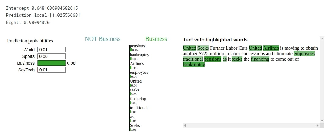
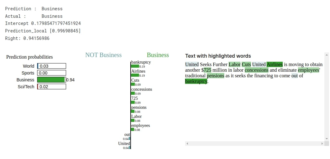
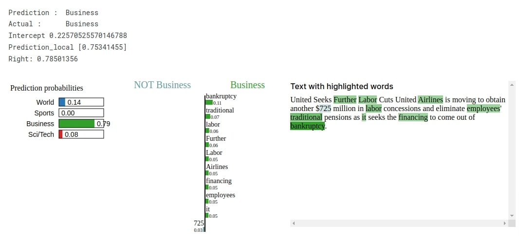
After defining a function, we randomly selected on text example from the test dataset and made predictions on it using our trained network. We have then printed the actual and predicted labels for the selected sample. We can notice that our model correctly predicts the category as 'Business'.
If you are new to LIME and want to learn about it in-depth then please feel free to check the below link where we have covered the algorithm and its uses in detail.
X_test_text, Y_test = [], []
for Y, X in test_dataset:
    X_test_text.append(X)
    Y_test.append(Y-1)

len(X_test_text)
from lime import lime_text
import numpy as np

explainer = lime_text.LimeTextExplainer(class_names=target_classes, verbose=True)

def make_predictions(X_batch_text):
    X = [vocab(tokenizer(text)) for text in X_batch_text]
    X = [tokens+([0]* (max_words-len(tokens))) if len(tokens)<max_words else tokens[:max_words] for tokens in X] ## Bringing all samples to max_words length.
    logits = rnn_classifier(torch.tensor(X, dtype=torch.int32))
    preds = F.softmax(logits, dim=-1)
    return preds.detach().numpy()

rng = np.random.RandomState(1)
idx = rng.randint(1, len(X_test_text))
X = [vocab(tokenizer(text)) for text in X_test_text[idx:idx+1]]
X = [tokens+([0]* (max_words-len(tokens))) if len(tokens)<max_words else tokens[:max_words] for tokens in X] ## Bringing all samples to max_words length.
preds = rnn_classifier(torch.tensor(X, dtype=torch.int32))
preds = F.softmax(preds, dim=-1)

print("Prediction : ", target_classes[preds.argmax()])
print("Actual :     ", target_classes[Y_test[idx]])
Below, we have called explain_instance() method with selected text example, prediction function, and target label for selected example to generate Explanation instance. Then, we have called show_in_notebook() method to generate a visualization showing an explanation. We can notice from the visualization that words like 'pensions', 'bankruptcy', 'airlines', 'employees', 'financing', etc are contributing to predicting category 'Business'.
explanation = explainer.explain_instance(X_test_text[idx], classifier_fn=make_predictions,
                                         labels=Y_test[idx:idx+1])
explanation.show_in_notebook()
Approach 2: Single RNN Layer (Tokens Per Text Example=50, Embeddings Length=50) 
Our approach in this section is exactly the same as our approach in the previous section with only a difference in the number of tokens used per text example. Our previous approach kept 25 tokens per text example whereas, in this section, we have kept 50 tokens per text example. The code is almost exactly the same as in our previous section.
Load Datasets And Create Data Loaders
Below, we have loaded the dataset again and created data loaders from it. We have set max_words to 50 this time to keep 50 tokens per text example.
from torch.utils.data import DataLoader
from torchtext.data.functional import to_map_style_dataset

train_dataset, test_dataset  = torchtext.datasets.AG_NEWS()
train_dataset, test_dataset  = to_map_style_dataset(train_dataset), to_map_style_dataset(test_dataset)

target_classes = ["World", "Sports", "Business", "Sci/Tech"]

max_words = 50

train_loader = DataLoader(train_dataset, batch_size=1024, collate_fn=vectorize_batch, shuffle=True)
test_loader  = DataLoader(test_dataset , batch_size=1024, collate_fn=vectorize_batch)
for X, Y in train_loader:
    print(X.shape, Y.shape)
    break
Define RNN Classification Network
Here, we have defined a network that we'll use for the text classification task in this section. The definition of a network is almost exactly the same as in the previous section with minor changes.
from torch import nn
from torch.nn import functional as F

embed_len = 50
hidden_dim = 50
n_layers=1

class RNNClassifier(nn.Module):
    def __init__(self):
        super(RNNClassifier, self).__init__()
        self.embedding_layer = nn.Embedding(num_embeddings=len(vocab), embedding_dim=embed_len)
        self.rnn = nn.RNN(input_size=embed_len, hidden_size=hidden_dim, num_layers=n_layers,
                          batch_first=True, nonlinearity="relu", dropout=0.2)
        self.linear = nn.Linear(hidden_dim, len(target_classes))

    def forward(self, X_batch):
        embeddings = self.embedding_layer(X_batch)
        output, hidden = self.rnn(embeddings, torch.randn(n_layers, len(X_batch), hidden_dim))
        return self.linear(output[:,-1])
Train Network
Now, we have trained our new network using exactly the same settings (15 epochs and learning rate of 0.001) that we have used in the previous approach. We'll be keeping our settings the same for all upcoming approaches as well. We can notice from the loss and accuracy getting printed after each epoch that our model is doing a good job.
from torch.optim import Adam

epochs = 15
learning_rate = 1e-3

loss_fn = nn.CrossEntropyLoss()
rnn_classifier = RNNClassifier()
optimizer = Adam(rnn_classifier.parameters(), lr=learning_rate)

TrainModel(rnn_classifier, loss_fn, optimizer, train_loader, test_loader, epochs)
Evaluate Network Performance
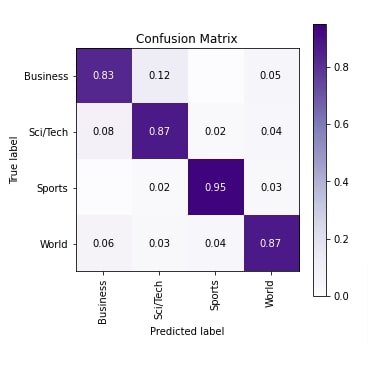
In this section, we have evaluated the performance of our network by calculating accuracy, classification report and confusion matrix on test predictions as usual. We can notice from the test accuracy that it has improved a bit from our previous approach.
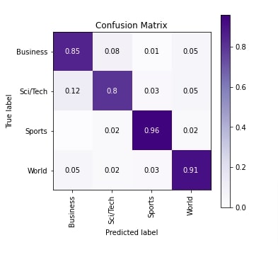
In the next cell after the below cell, we have plotted the confusion matrix which indicates that our model is doing a good job at classifying text documents of categories Sports and World compared to categories Business and Sci/Tech.
from sklearn.metrics import accuracy_score, classification_report, confusion_matrix

Y_actual, Y_preds = MakePredictions(rnn_classifier, test_loader)

print("Test Accuracy : {}".format(accuracy_score(Y_actual, Y_preds)))
print("\nClassification Report : ")
print(classification_report(Y_actual, Y_preds, target_names=target_classes))
print("\nConfusion Matrix : ")
print(confusion_matrix(Y_actual, Y_preds))
from sklearn.metrics import confusion_matrix
import scikitplot as skplt
import matplotlib.pyplot as plt
import numpy as np

skplt.metrics.plot_confusion_matrix([target_classes[i] for i in Y_actual], [target_classes[i] for i in Y_preds],
                                    normalize=True,
                                    title="Confusion Matrix",
                                    cmap="Purples",
                                    hide_zeros=True,
                                    figsize=(5,5)
                                    );
plt.xticks(rotation=90);
Explain Network Predictions Using LIME Algorithm
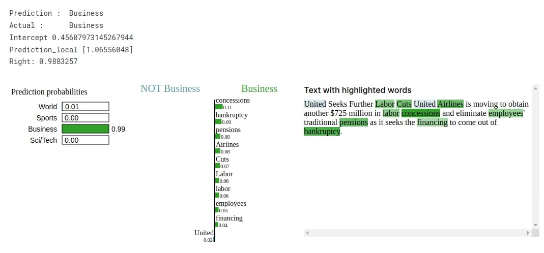
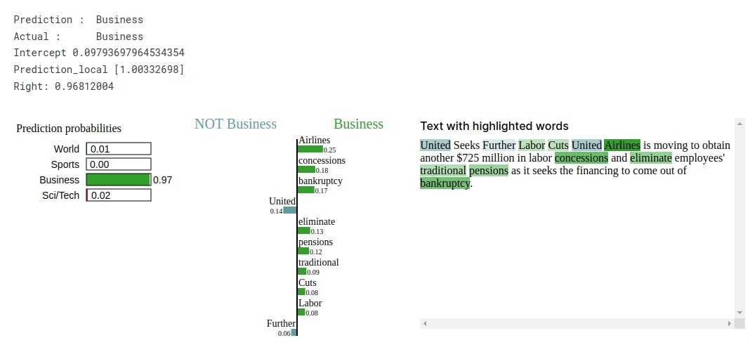
In this section, we have again tried to explain the prediction made by our network using LIME algorithm. We have randomly selected a sample and our model correctly predicts the target label as 'Business' for it. We can notice from the visualization that words like 'concessions', 'bankruptcy', 'pensions', 'labor', 'employees', 'financing', etc are contributing to predicting 'Business' category.
from lime import lime_text
import numpy as np

explainer = lime_text.LimeTextExplainer(class_names=target_classes, verbose=True)

rng = np.random.RandomState(1)
idx = rng.randint(1, len(X_test_text))
X = [vocab(tokenizer(text)) for text in X_test_text[idx:idx+1]]
X = [tokens+([0]* (max_words-len(tokens))) if len(tokens)<max_words else tokens[:max_words] for tokens in X] ## Bringing all samples to max_words length.
preds = rnn_classifier(torch.tensor(X, dtype=torch.int32))
preds = F.softmax(preds, dim=-1)

print("Prediction : ", target_classes[preds.argmax()])
print("Actual :     ", target_classes[Y_test[idx]])

explanation = explainer.explain_instance(X_test_text[idx], classifier_fn=make_predictions,
                                         labels=Y_test[idx:idx+1])
explanation.show_in_notebook()
Approach 3: Multiple RNN Layers (Tokens Per Text Example=50, Embeddings Length=50) 
All our previous approaches used a single recurrent layer in the network. As a part of our approach in this section, we have stacked 3 recurrent layers together. As we have stacked more recurrent layers, it should hopefully help better classify text documents. The code in this section is almost the same as our code from previous approaches with very minor changes.
Define RNN Classification Network
Below, we have defined our network which has exactly the same code as our previous networks with only a change in value given to num_layers parameter of RNN() constructor. We have set the value of the parameter to 3 to ask it to stack 3 recurrent layers. The rest of the code is the same as our previous networks.
After defining the network, we have also initialized it and printed the shape of weights/biases of layers of the network.
from torch import nn
from torch.nn import functional as F

embed_len = 50
hidden_dim = 50
n_layers=3

class RNNClassifier(nn.Module):
    def __init__(self):
        super(RNNClassifier, self).__init__()
        self.embedding_layer = nn.Embedding(num_embeddings=len(vocab), embedding_dim=embed_len)
        self.rnn = nn.RNN(input_size=embed_len, hidden_size=hidden_dim, num_layers=n_layers, batch_first=True)
        self.linear = nn.Linear(hidden_dim, len(target_classes))

    def forward(self, X_batch):
        embeddings = self.embedding_layer(X_batch)
        output, hidden = self.rnn(embeddings, torch.randn(n_layers, len(X_batch), hidden_dim))
        return self.linear(output[:,-1])
rnn_classifier = RNNClassifier()

rnn_classifier
for layer in rnn_classifier.children():
    print("Layer : {}".format(layer))
    print("Parameters : ")
    for param in layer.parameters():
        print(param.shape)
    print()
Train Network
In this section, we have trained our 3 recurrent layers network with the same settings that we have been using for all our approaches. We can notice from the loss and accuracy value getting printed after each epoch that our model seems to be doing a decent job at the task.
from torch.optim import Adam

epochs = 15
learning_rate = 1e-3

loss_fn = nn.CrossEntropyLoss()
rnn_classifier = RNNClassifier()
optimizer = Adam(rnn_classifier.parameters(), lr=learning_rate)

TrainModel(rnn_classifier, loss_fn, optimizer, train_loader, test_loader, epochs)
Evaluate Network Performance
In this section, we have again evaluated various ML metrics on test predictions. We can notice from the accuracy that it's a little less compared to our previous approach. It seems from this experiment that multiple recurrent layers are not giving better accuracy compared to a single recurrent layer. Though trying different hyperparameters combinations might improve results.
from sklearn.metrics import accuracy_score, classification_report, confusion_matrix

Y_actual, Y_preds = MakePredictions(rnn_classifier, test_loader)

print("Test Accuracy : {}".format(accuracy_score(Y_actual, Y_preds)))
print("\nClassification Report : ")
print(classification_report(Y_actual, Y_preds, target_names=target_classes))
print("\nConfusion Matrix : ")
print(confusion_matrix(Y_actual, Y_preds))
from sklearn.metrics import confusion_matrix
import scikitplot as skplt
import matplotlib.pyplot as plt
import numpy as np

skplt.metrics.plot_confusion_matrix([target_classes[i] for i in Y_actual], [target_classes[i] for i in Y_preds],
                                    normalize=True,
                                    title="Confusion Matrix",
                                    cmap="Purples",
                                    hide_zeros=True,
                                    figsize=(5,5)
                                    );
plt.xticks(rotation=90);
Explain Network Predictions Using LIME Algorithm
In this section, we have explained prediction using LIME algorithm. We have randomly selected a test example and our model correctly predicts the target label as 'Business' for it. The words like 'bankruptcy', 'airlines', 'cuts', 'concessions', 'pensions', 'labor', 'employees', etc seems to be contributing to predicting category as 'Business'.
from lime import lime_text
import numpy as np

explainer = lime_text.LimeTextExplainer(class_names=target_classes, verbose=True)

rng = np.random.RandomState(1)
idx = rng.randint(1, len(X_test_text))
X = [vocab(tokenizer(text)) for text in X_test_text[idx:idx+1]]
X = [tokens+([0]* (max_words-len(tokens))) if len(tokens)<max_words else tokens[:max_words] for tokens in X] ## Bringing all samples to max_words length.
preds = rnn_classifier(torch.tensor(X, dtype=torch.int32))
preds = F.softmax(preds, dim=-1)

print("Prediction : ", target_classes[preds.argmax()])
print("Actual :     ", target_classes[Y_test[idx]])

explanation = explainer.explain_instance(X_test_text[idx], classifier_fn=make_predictions,
                                         labels=Y_test[idx:idx+1])
explanation.show_in_notebook()
Approach 4: Stacking Multiple RNN Layers (Tokens Per Text Example=50, Embeddings Length=50) 
Our approach in this section is the same as our approach in the previous section of stacking multiple recurrent layers but the output size of the recurrent layer is different in this approach. In the previous approach, the output size of all recurrent layers was the same. The majority of the code in the section is a repeat of previous sections.
Define RNN Classification Network
Below, we have defined the network that we'll use in this section. We have defined 3 recurrent layers in this section with output sizes of 50, 60, and 75. The output of the embedding layer is given to the first recurrent layer, the output of the first recurrent layer is given to the second, and the output of the second recurrent layer is given to the third one. The output of the last recurrent layer is given to the linear layer whose output will be a prediction of the network.
After defining the network, we initialized it and printed the shapes of weights/biases of different layers of the network.
from torch import nn
from torch.nn import functional as F

embed_len = 50
hidden_dim1 = 50
hidden_dim2 = 60
hidden_dim3 = 75
n_layers=1

class RNNClassifier(nn.Module):
    def __init__(self):
        super(RNNClassifier, self).__init__()
        self.embedding_layer = nn.Embedding(num_embeddings=len(vocab), embedding_dim=embed_len)
        self.rnn1 = nn.RNN(input_size=embed_len, hidden_size=hidden_dim1, num_layers=1, batch_first=True)
        self.rnn2 = nn.RNN(input_size=hidden_dim1, hidden_size=hidden_dim2, num_layers=1, batch_first=True)
        self.rnn3 = nn.RNN(input_size=hidden_dim2, hidden_size=hidden_dim3, num_layers=1, batch_first=True)
        self.linear = nn.Linear(hidden_dim3, len(target_classes))

    def forward(self, X_batch):
        embeddings = self.embedding_layer(X_batch)
        output, hidden = self.rnn1(embeddings, torch.randn(n_layers, len(X_batch), hidden_dim1))
        output, hidden = self.rnn2(output, torch.randn(n_layers, len(X_batch), hidden_dim2))
        output, hidden = self.rnn3(output, torch.randn(n_layers, len(X_batch), hidden_dim3))
        return self.linear(output[:,-1])
rnn_classifier = RNNClassifier()

rnn_classifier
for layer in rnn_classifier.children():
    print("Layer : {}".format(layer))
    print("Parameters : ")
    for param in layer.parameters():
        print(param.shape)
    print()
Train Network
In this section, we have trained our new network using the same settings that we have been using for all our approaches. The loss and accuracy getting printed after completion of each epoch hints that the model is doing a good job at the text classification task.
from torch.optim import Adam

epochs = 15
learning_rate = 1e-3

loss_fn = nn.CrossEntropyLoss()
rnn_classifier = RNNClassifier()
optimizer = Adam(rnn_classifier.parameters(), lr=learning_rate)

TrainModel(rnn_classifier, loss_fn, optimizer, train_loader, test_loader, epochs)
Evaluate Network Performance
Here, we have evaluated the performance of our network from this approach by calculating various ML metrics. We can notice from the accuracy of the model that it is a little more compared to our previous approach of using the same length multiple recurrent layers.
from sklearn.metrics import accuracy_score, classification_report, confusion_matrix

Y_actual, Y_preds = MakePredictions(rnn_classifier, test_loader)

print("Test Accuracy : {}".format(accuracy_score(Y_actual, Y_preds)))
print("\nClassification Report : ")
print(classification_report(Y_actual, Y_preds, target_names=target_classes))
print("\nConfusion Matrix : ")
print(confusion_matrix(Y_actual, Y_preds))
from sklearn.metrics import confusion_matrix
import scikitplot as skplt
import matplotlib.pyplot as plt
import numpy as np

skplt.metrics.plot_confusion_matrix([target_classes[i] for i in Y_actual], [target_classes[i] for i in Y_preds],
                                    normalize=True,
                                    title="Confusion Matrix",
                                    cmap="Purples",
                                    hide_zeros=True,
                                    figsize=(5,5)
                                    );
plt.xticks(rotation=90);
Explain Network Predictions Using LIME Algorithm
In this section, we have explained the prediction made by our network from this section using LIME algorithm. The model correctly predicts the target label as 'Business' for the randomly selected test sample. The words like 'concessions', 'bankruptcy', 'pensions', 'cuts', 'labor', etc are contributing to prediction.
from lime import lime_text
import numpy as np

explainer = lime_text.LimeTextExplainer(class_names=target_classes, verbose=True)

rng = np.random.RandomState(1)
idx = rng.randint(1, len(X_test_text))
X = [vocab(tokenizer(text)) for text in X_test_text[idx:idx+1]]
X = [tokens+([0]* (max_words-len(tokens))) if len(tokens)<max_words else tokens[:max_words] for tokens in X] ## Bringing all samples to max_words length.
preds = rnn_classifier(torch.tensor(X, dtype=torch.int32))
preds = F.softmax(preds, dim=-1)

print("Prediction : ", target_classes[preds.argmax()])
print("Actual :     ", target_classes[Y_test[idx]])

explanation = explainer.explain_instance(X_test_text[idx], classifier_fn=make_predictions,
                                         labels=Y_test[idx:idx+1])
explanation.show_in_notebook()
Approach 5: Multiple Bidirectional RNN Layers (Tokens Per Text Example=50, Embeddings Length=50) 
Our approach in this section is the same as our third approach where we had used 3 recurrent layers of the same output size. The only difference in this approach is that we have used bidirectional recurrent layers. The bidirectional recurrent layers work exactly like unidirectional but it works in forward and backward directions both. When we give the recurrent layer 50 tokens (50 words of our text example), the cycle of applying the recurrent layer will go through 50 tokens in both directions (start to end and end to start). As the bidirectional recurrent layer performs a function in both directions, the output shape of it will be 2 times the output shape of the unidirectional recurrent layer as we have an output for both directions. Our code in this section is the same as our code from the third approach with minor parameter value change.
Define RNN Classification Network
Below, we have defined the network that we'll be using for our task. Our network is the same as the one from the third approach with minor changes. We have set bidirectional parameter of RNN() constructor to True. The input units of the linear layer are 2 times the output units of the recurrent layer as it is a bidirectional layer.
After defining the network, we initialized it and printed the shapes of weights/biases of layers for information purposes.
from torch import nn
from torch.nn import functional as F

embed_len = 50
hidden_dim = 50
n_layers=3

class RNNClassifier(nn.Module):
    def __init__(self):
        super(RNNClassifier, self).__init__()
        self.embedding_layer = nn.Embedding(num_embeddings=len(vocab), embedding_dim=embed_len)
        self.rnn = nn.RNN(input_size=embed_len, hidden_size=hidden_dim, num_layers=n_layers,
                          batch_first=True, bidirectional=True) ## Bidirectional RNN
        self.linear = nn.Linear(2*hidden_dim, len(target_classes)) ## Input dimension are 2 times hidden dimensions due to bidirectional results

    def forward(self, X_batch):
        embeddings = self.embedding_layer(X_batch)
        output, hidden = self.rnn(embeddings, torch.randn(2*n_layers, len(X_batch), hidden_dim))
        return self.linear(output[:,-1])
rnn_classifier = RNNClassifier()

rnn_classifier
for layer in rnn_classifier.children():
    print("Layer : {}".format(layer))
    print("Parameters : ")
    for param in layer.parameters():
        print(param.shape)
    print()
Train Network
In this section, we have trained our network using the same settings that we have used for all our previous approaches. We can notice from the loss and accuracy values getting printed after each epoch that our model is doing a good job at the task.
from torch.optim import Adam

epochs = 25
learning_rate = 1e-4

loss_fn = nn.CrossEntropyLoss()
rnn_classifier = RNNClassifier()
optimizer = Adam(rnn_classifier.parameters(), lr=learning_rate)

TrainModel(rnn_classifier, loss_fn, optimizer, train_loader, test_loader, epochs)
Evaluate Network Performance
Here, we have evaluated various ML metrics for our network on test predictions. We can notice from the accuracy that our model from this approach has the least accuracy.
from sklearn.metrics import accuracy_score, classification_report, confusion_matrix

Y_actual, Y_preds = MakePredictions(rnn_classifier, test_loader)

print("Test Accuracy : {}".format(accuracy_score(Y_actual, Y_preds)))
print("\nClassification Report : ")
print(classification_report(Y_actual, Y_preds, target_names=target_classes))
print("\nConfusion Matrix : ")
print(confusion_matrix(Y_actual, Y_preds))
from sklearn.metrics import confusion_matrix
import scikitplot as skplt
import matplotlib.pyplot as plt
import numpy as np

skplt.metrics.plot_confusion_matrix([target_classes[i] for i in Y_actual], [target_classes[i] for i in Y_preds],
                                    normalize=True,
                                    title="Confusion Matrix",
                                    cmap="Purples",
                                    hide_zeros=True,
                                    figsize=(5,5)
                                    );
plt.xticks(rotation=90);
Explain Network Predictions Using LIME Algorithm
Here, we have again tried to explain the prediction of our network using LIME algorithm. The network correctly predicts the target category as 'Business' for the selected test example through the probability is a little less. The words like 'bankruptcy', 'labor', 'financing', 'employees', etc are contributing to predicting 'Business' category.
from lime import lime_text
import numpy as np

explainer = lime_text.LimeTextExplainer(class_names=target_classes, verbose=True)

rng = np.random.RandomState(1)
idx = rng.randint(1, len(X_test_text))
X = [vocab(tokenizer(text)) for text in X_test_text[idx:idx+1]]
X = [tokens+([0]* (max_words-len(tokens))) if len(tokens)<max_words else tokens[:max_words] for tokens in X] ## Bringing all samples to max_words length.
preds = rnn_classifier(torch.tensor(X, dtype=torch.int32))
preds = F.softmax(preds, dim=-1)

print("Prediction : ", target_classes[preds.argmax()])
print("Actual :     ", target_classes[Y_test[idx]])

explanation = explainer.explain_instance(X_test_text[idx], classifier_fn=make_predictions,
                                         labels=Y_test[idx:idx+1])
explanation.show_in_notebook()
7. Summary of Results And Suggestions 
In this section, we have simply summarized the results of various approaches for easier comparisons. We have also suggested a few more things to try which might improve performance further.
| Approach | Test Accuracy |
|---|---|
| Approach 1: Single RNN Layer (Tokens Per Text Example=25, Embeddings Length=50) | 87.28 % |
| Approach 2: Single RNN Layer (Tokens Per Text Example=50, Embeddings Length=50) | 87.98 % |
| Approach 3: Multiple RNN Layers (Tokens Per Text Example=50, Embeddings Length=50) | 86.77 % |
| Approach 4: Stacking Multiple RNN Layers (Tokens Per Text Example=50, Embeddings Length=50) | 87.86 % |
| Approach 5: Multiple Bidirectional RNN Layers (Tokens Per Text Example=50, Embeddings Length=50) | 74.84 % |
Further Suggestions
Below is a list of things that can be tried to further improve the performance of the network.
- Try different token sizes.
- Try different embedding lengths.
- Try different output/hidden sizes of recurrent layers.
- Train model for more epochs.
- Try different weight initializers.
- Try different values of dropout with recurrent layers.
- Add a few more liner layers after recurrent layers.
Apart from the above-mentioned suggestions, there can be other things that can help improve the performance further but they need to be tried.
This ends our small tutorial explaining how we can design RNN for text classification tasks using PyTorch. Please feel free to let us know your views in the comments section.
References
 Sunny Solanki
Sunny Solanki
Intro: Software Developer | Youtuber | Bonsai Enthusiast
About: Sunny Solanki holds a bachelor's degree in Information Technology (2006-2010) from L.D. College of Engineering. Post completion of his graduation, he has 8.5+ years of experience (2011-2019) in the IT Industry (TCS). His IT experience involves working on Python & Java Projects with US/Canada banking clients. Since 2020, he’s primarily concentrating on growing CoderzColumn.
His main areas of interest are AI, Machine Learning, Data Visualization, and Concurrent Programming. He has good hands-on with Python and its ecosystem libraries.
Apart from his tech life, he prefers reading biographies and autobiographies. And yes, he spends his leisure time taking care of his plants and a few pre-Bonsai trees.
Contact: sunny.2309@yahoo.in


![YouTube Subscribe]() Comfortable Learning through Video Tutorials?
Comfortable Learning through Video Tutorials?
If you are more comfortable learning through video tutorials then we would recommend that you subscribe to our YouTube channel.
![Need Help]() Stuck Somewhere? Need Help with Coding? Have Doubts About the Topic/Code?
Stuck Somewhere? Need Help with Coding? Have Doubts About the Topic/Code?
 Stuck Somewhere? Need Help with Coding? Have Doubts About the Topic/Code?
When going through coding examples, it's quite common to have doubts and errors.
If you have doubts about some code examples or are stuck somewhere when trying our code, send us an email at coderzcolumn07@gmail.com. We'll help you or point you in the direction where you can find a solution to your problem.
You can even send us a mail if you are trying something new and need guidance regarding coding. We'll try to respond as soon as possible.
![Share Views]() Want to Share Your Views? Have Any Suggestions?
Want to Share Your Views? Have Any Suggestions?
 Want to Share Your Views? Have Any Suggestions?
If you want to
- provide some suggestions on topic
- share your views
- include some details in tutorial
- suggest some new topics on which we should create tutorials/blogs
 pytorch, rnn, text-classification