PyTorch LSTM For Text Classification Tasks (Word Embeddings)
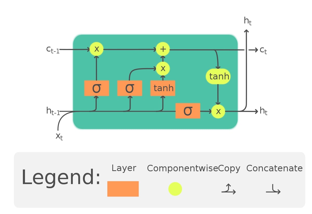
Long Short-Term Memory (LSTM) networks are a type of recurrent neural network that is better at remembering sequence order compared to simple RNN. The traditional RNN can not learn sequence order for very long sequences in practice even though in theory it seems to be possible. It suffers from a problem called vanishing gradient. On the other hand, an advanced version of RNN like LSTM can remember the order of sequences for very long sequences and solves vanishing gradient problem to an extent. Here, by sequences, we mean data that has order like time-series data, speech data, text data, etc. LSTM helps us capture order better compared to our dense layer networks. Below, we have included an image of one cell of LSTM. Inside of LSTM layer, many LSTM cells like those below are laid next to each other to remember the sequence of data.
As a part of this tutorial, we are going to explain how we can design various LSTM networks using PyTorch to solve a text classification task. We have tried different approaches to using LSTM networks to solve the tasks. The tutorial does not cover the theoretical aspect of LSTM. Please check the below link if you are looking for it.
We also recommend that readers go through our tutorial on designing PyTorch RNN networks for text classification tasks that use vanilla RNN layers for text classification.
Below, we have listed important sections of tutorial to give an overview of the material covered.
Important Sections Of Tutorial
- Populate Vocabulary
- Approach 1: Single LSTM Layer (Tokens Per Text Example=25, Embeddings Length=50, LSTM Output=75)
- Load Dataset And Create Data Loaders
- Define LSTM Network
- Train Network
- Evaluate Network Performance
- Explain Predictions Using LIME Algorithm
- Approach 2: Single LSTM Layer (Tokens Per Text Example=50, Embeddings Length=50, LSTM Output=75)
- Approach 3: Multiple LSTM Layers (Tokens Per Text Example=50, Embeddings Length=50, LSTM Output=75)
- Approach 4: Stacking Multiple LSTM Layers (Tokens Per Text Example=50, Embeddings Length=50, LSTM Output=75)
- Approach 5: Multiple Bidirectional LSTM Layers (Tokens Per Text Example=50, Embeddings Length=50, LSTM Output=75)
- Results Summary and Suggestions
Below, we have imported the necessary libraries and printed the versions that we have used in our tutorial.
import torch

print("PyTorch Version : {}".format(torch.__version__))
import torchtext

print("TorchText Version : {}".format(torchtext.__version__))
1. Populate Vocabulary 
In this section, we have populated a vocabulary with the tokens of the text of the dataset. The vocabulary is a simple mapping of tokens to an integer index. Index starting from integer 1 will be used to represent each token.
Below, we have first loaded AG NEWS dataset available from datasets sub-module of torchtext library. The dataset has news text examples for four different categories(["World", "Sports", "Business", "Sci/Tech"]). The dataset is already divided into train and test sets.
from torch.utils.data import DataLoader

train_dataset, test_dataset  = torchtext.datasets.AG_NEWS()
Below, we have first declared a tokenizer. The tokenizer is a function that splits text into a list of tokens. These tokens are generally words but they can be punctuation and symbols as well.
After defining tokenizer, we have populated vocabulary using build_vocab_from_iterator() function available from vocab sub-module of torchtext library. As the name of the function suggests, it creates vocabulary from an iterator. We have created a simple iterator named build_vocabulary() that takes a list of datasets as input. It then loops through each dataset and each text example of the dataset yielding a list of tokens for each text example using a tokenizer. We have called build_vocab_from_iterator() function by giving this iterator with train and test datasets as arguments. The build_vocab_from_iterator() function will populate vocabulary from tokens yielded by this iterator. We have set min_freq parameter to 1 which indicates that we'll keep all words whose word frequency is at least one.
After populating the vocabulary, we have also printed the length of the vocabulary. We have also explained with a simple example how we can convert text to a list of tokens and then a list of indexes.
from torchtext.data import get_tokenizer
from torchtext.vocab import build_vocab_from_iterator

tokenizer = get_tokenizer("basic_english")

def build_vocabulary(datasets):
    for dataset in datasets:
        for _, text in dataset:
            yield tokenizer(text)

vocab = build_vocab_from_iterator(build_vocabulary([train_dataset, test_dataset]), min_freq=1, specials=["<UNK>"])
vocab.set_default_index(vocab["<UNK>"])
len(vocab)
tokens = tokenizer("Hello how are you?, Welcome to CoderzColumn!!")
indexes = vocab(tokens)

tokens, indexes
vocab["<UNK>"] ## Coderzcolumn word is mapped to unknown as it's new and not present in vocabulary
Approach 1: Single LSTM Layer (Tokens Per Text Example=25, Embeddings Length=50, LSTM Output=75) 
In our first approach to using LSTM network for the text classification tasks, we have developed a simple neural network with one LSTM layer which has an output length of 75. We have used word embeddings approach for encoding text using vocabulary populated earlier. We have trained the network, evaluated its performance by calculating various ML metrics, and also explained network predictions using LIME algorithm.
Load Dataset And Create Data Loaders
In this section, we have first loaded our datasets (train and test) and then created data loaders from them which will be used during the training process to loop through training data in batches.
Below, we have first loaded our datasets. Then, we have created data loaders using these datasets. We have provided a batch size of 1024 samples per batch. We have also provided vectorization function to collate_fn argument of the DataLoader() constructors. This function takes batches of text and their respective target labels. It then tokenizes these text examples and maps tokens to indexes using our vocabulary. This function will be applied to all batches of data.
We have set max_words to 25 which is to inform data loaders that we want to keep a maximum of 25 tokens per text example. If the text example has tokens less than it then it'll be appended with 0s and more than it then it'll be truncated after the first 25 tokens.
At last, we return torch tensors from the vectorize_batch() function. The function returns indexes for each text example and their respective target labels as torch tensors. Please make a NOTE that we have deducted 1 from the original target labels as they are in range 1-4 and we want labels in range 0-3.
from torch.utils.data import DataLoader
from torchtext.data.functional import to_map_style_dataset

train_dataset, test_dataset  = torchtext.datasets.AG_NEWS()
train_dataset, test_dataset  = to_map_style_dataset(train_dataset), to_map_style_dataset(test_dataset)

target_classes = ["World", "Sports", "Business", "Sci/Tech"]

max_words = 25

def vectorize_batch(batch):
    Y, X = list(zip(*batch))
    X = [vocab(tokenizer(text)) for text in X] ## Tokenize and map tokens to indexes
    X = [tokens+([0]* (max_words-len(tokens))) if len(tokens)<max_words else tokens[:max_words] for tokens in X] ## Bringing all samples to max_words length.

    return torch.tensor(X, dtype=torch.int32), torch.tensor(Y) - 1 ## We have deducted 1 from target names to get them in range [0,1,2,3] from [1,2,3,4]


train_loader = DataLoader(train_dataset, batch_size=1024, collate_fn=vectorize_batch, shuffle=True)
test_loader  = DataLoader(test_dataset , batch_size=1024, collate_fn=vectorize_batch)
for X, Y in train_loader:
    print(X.shape, Y.shape)
    break
Define LSTM Network
In this section, we have defined our LSTM network which consists of 3 layers.
- Embedding Layer
- LSTM Layer
- Linear Layer
The Embedding Layer takes the input list of indexes generated by the vectorization function. We have initialized a layer with a number of embeddings equal to the length of vocabulary and embedding length to 50. This initialization will create a weight tensor of shape (vocab_len, embed_len) which has an embedding vector of length 50 for each token of vocabulary. The layer is responsible for mapping the index of each token to a float vector of length 50 because we have set the embedding length to 50. This layer takes tensor of shape (batch_size, max_tokens) and outputs tensor of shape (batch_size, max_tokens, embed_len). Each token gets assigned its respective embedding vector based on the index value by this layer. If you are new to the concept of word embeddings then we recommend that you go through the below tutorial as it'll help you understand it in detail.
The LSTM Layer takes embeddings generated by the embedding layer as input. We have initialized LSTM layer with a number of subsequent LSTM layers set to 1, output/hidden shape of LSTM set to 75 and input shape set to the same as embedding length. The LSTM layer internally loops through embeddings of each text example and generates hidden and output tensors. The layer is basically a loop through embeddings of single text examples one by one generating output after each token. It takes the hidden state and the carry as input which are generally random numbers and required by first token only. The hidden and carry tensors for subsequent tokens are generated by the LSTM function. The input to LSTM is of shape (batch_size, max_tokens, embed_len) and output of shape (batch_size, max_tokens, hidden_dim). Please make a NOTE that we have used only a single LSTM layer in this approach. We'll be using multiple in our upcoming examples.
The last layer of the network is Linear layer which has 4 output units that are the same as a number of target classes. It takes the last input of the LSTM layer and returns the prediction of the network. Please take a look at the input given to Linear Layer in the forward pass. We have given the last output of each example generated by LSTM. The output of LSTM is the output of each token of an example but we want the output of the last token for each example which generally has captured the context of the whole example.
After defining a network, we initialized it, printed the shape of weights/biases of each layer of the network, and performed a forward pass through random data to verify the network.
Please take a look at the below tutorial if you are new to PyTorch and want to learn how to create a neural network using it first. It'll help you sail through this tutorial faster.
from torch import nn
from torch.nn import functional as F

embed_len = 50
hidden_dim = 75
n_layers=1

class LSTMClassifier(nn.Module):
    def __init__(self):
        super(LSTMClassifier, self).__init__()
        self.embedding_layer = nn.Embedding(num_embeddings=len(vocab), embedding_dim=embed_len)
        self.lstm = nn.LSTM(input_size=embed_len, hidden_size=hidden_dim, num_layers=n_layers, batch_first=True)
        self.linear = nn.Linear(hidden_dim, len(target_classes))

    def forward(self, X_batch):
        embeddings = self.embedding_layer(X_batch)
        hidden, carry = torch.randn(n_layers, len(X_batch), hidden_dim), torch.randn(n_layers, len(X_batch), hidden_dim)
        output, (hidden, carry) = self.lstm(embeddings, (hidden, carry))
        return self.linear(output[:,-1])
lstm_classifier = LSTMClassifier()

lstm_classifier
for layer in lstm_classifier.children():
    print("Layer : {}".format(layer))
    print("Parameters : ")
    for param in layer.parameters():
        print(param.shape)
    print()
out = lstm_classifier(torch.randint(0, len(vocab), (1024, max_words)))

out.shape
Train Network
In this section, we have trained a network that we defined in the previous section. In order to train the network, we have defined a function that will perform training when called.
The function takes model, loss function, optimizer, train data loader, validation data loader, and a number of epochs as input. It then executes a training loop number of epochs time. For each epoch, it loops through whole training data in batches using a train data loader. For each batch of data, it performs a forward pass to make predictions, calculates loss, calculates gradients, and updates network weights. It records loss for each batch and prints the average loss of all batches of the epoch at the end. It also calculates validation loss and accuracy using a helper function and prints it as well.
from tqdm import tqdm
from sklearn.metrics import accuracy_score
import gc

def CalcValLossAndAccuracy(model, loss_fn, val_loader):
    with torch.no_grad():
        Y_shuffled, Y_preds, losses = [],[],[]
        for X, Y in val_loader:
            preds = model(X)
            loss = loss_fn(preds, Y)
            losses.append(loss.item())

            Y_shuffled.append(Y)
            Y_preds.append(preds.argmax(dim=-1))

        Y_shuffled = torch.cat(Y_shuffled)
        Y_preds = torch.cat(Y_preds)

        print("Valid Loss : {:.3f}".format(torch.tensor(losses).mean()))
        print("Valid Acc  : {:.3f}".format(accuracy_score(Y_shuffled.detach().numpy(), Y_preds.detach().numpy())))


def TrainModel(model, loss_fn, optimizer, train_loader, val_loader, epochs=10):
    for i in range(1, epochs+1):
        losses = []
        for X, Y in tqdm(train_loader):
            Y_preds = model(X) ## Make Predictions

            loss = loss_fn(Y_preds, Y) ## Calculate Loss
            losses.append(loss.item())

            optimizer.zero_grad() ## Clear previously calculated gradients
            loss.backward() ## Calculates Gradients
            optimizer.step() ## Update network weights.

        print("Train Loss : {:.3f}".format(torch.tensor(losses).mean()))
        CalcValLossAndAccuracy(model, loss_fn, val_loader)
Below, we are actually training our network. We have initialized a number of epochs to 10 and the learning rate to 0.001. Then, we have initialized cross entropy loss function, our LSTM Text Classifier and Adam optimizer. At last, we have called our training function with the necessary arguments to perform training. We can notice from the loss and accuracy value getting printed after each epoch that our model is doing a good job at the classification task.
from torch.optim import Adam

epochs = 10
learning_rate = 1e-3

loss_fn = nn.CrossEntropyLoss()
lstm_classifier = LSTMClassifier()
optimizer = Adam(lstm_classifier.parameters(), lr=learning_rate)

TrainModel(lstm_classifier, loss_fn, optimizer, train_loader, test_loader, epochs)
Evaluate Network Performance
In this section, we have evaluated the performance of our network by calculating ML metrics like accuracy, classification report (precision, recall, and f1-score per target class) and confusion matrix on test predictions. We have created a helper function that takes the model and data loader as input and returns predictions. We can notice from the accuracy score that our model seems to have done a good job at the text classification task.
We have used various functions available from scikit-learn to calculate ML Metrics. Please feel free to check the below link if you want to learn about various ML metrics available from sklearn in-depth.
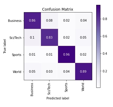
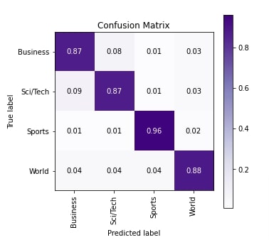
We have also created a visualization of the confusion matrix using scikit-plot. We can notice from the visualization that our model seems to be doing a good job for Sports and World categories compared to Business and Sci/Tech.
Please feel free to check the below link if you want to learn about scikit-plot and various ML metrics visualizations available from it.
def MakePredictions(model, loader):
    Y_shuffled, Y_preds = [], []
    for X, Y in loader:
        preds = model(X)
        Y_preds.append(preds)
        Y_shuffled.append(Y)
    gc.collect()
    Y_preds, Y_shuffled = torch.cat(Y_preds), torch.cat(Y_shuffled)

    return Y_shuffled.detach().numpy(), F.softmax(Y_preds, dim=-1).argmax(dim=-1).detach().numpy()

Y_actual, Y_preds = MakePredictions(lstm_classifier, test_loader)
from sklearn.metrics import accuracy_score, classification_report, confusion_matrix

print("Test Accuracy : {}".format(accuracy_score(Y_actual, Y_preds)))
print("\nClassification Report : ")
print(classification_report(Y_actual, Y_preds, target_names=target_classes))
print("\nConfusion Matrix : ")
print(confusion_matrix(Y_actual, Y_preds))
from sklearn.metrics import confusion_matrix
import scikitplot as skplt
import matplotlib.pyplot as plt
import numpy as np

skplt.metrics.plot_confusion_matrix([target_classes[i] for i in Y_actual], [target_classes[i] for i in Y_preds],
                                    normalize=True,
                                    title="Confusion Matrix",
                                    cmap="Purples",
                                    hide_zeros=True,
                                    figsize=(5,5)
                                    );
plt.xticks(rotation=90);
Explain Predictions Using LIME Algorithm
In this section, we have explained the predictions made by our model using LIME algorithm which is a commonly used library to explain predictions of black-box neural network models. It let us create a visualization explaining words that contributed to predicting a particular target label/category.
If you are new to LIME and have no background on it then we recommend that you go through the below link to understand it.
Below, we have simply loaded samples of the test dataset and their target labels.
X_test_text, Y_test = [], []
for Y, X in test_dataset:
    X_test_text.append(X)
    Y_test.append(Y-1)

len(X_test_text)
In order to explain predictions using LIME, we need to create an instance of LimeTextExplainer first. Then, we need to call explain_instance() method on it to create Explanation object which has explanation details. At last, we need to call show_in_notebook() method on Explanation object to create a visualization showing an explanation that has words highlighted from the text that contributed to predicting a particular target label.
Below, we have first initialized LimeTextExplainer. Then, we have defined a helper function that takes a list of text examples as input and returns their predicted probabilities. The function performs tokenizing and vectorization of text before giving it to the network to make predictions.
Then, we randomly selected a text example from the test dataset. We have made predictions on that example using our train model. Our model correctly predicts the target category as Business for it.
from lime import lime_text
import numpy as np

explainer = lime_text.LimeTextExplainer(class_names=target_classes, verbose=True) ## Define Explainer

def make_predictions(X_batch_text): ## Prediction Function
    X = [vocab(tokenizer(text)) for text in X_batch_text]
    X = [tokens+([0]* (max_words-len(tokens))) if len(tokens)<max_words else tokens[:max_words] for tokens in X] ## Bringing all samples to max_words length.
    logits = lstm_classifier(torch.tensor(X, dtype=torch.int32))
    preds = F.softmax(logits, dim=-1)
    return preds.detach().numpy()

## Randomly Select test example and make prediction on it.
rng = np.random.RandomState(1)
idx = rng.randint(1, len(X_test_text))
X = [vocab(tokenizer(text)) for text in X_test_text[idx:idx+1]]
X = [tokens+([0]* (max_words-len(tokens))) if len(tokens)<max_words else tokens[:max_words] for tokens in X] ## Bringing all samples to max_words length.
preds = lstm_classifier(torch.tensor(X, dtype=torch.int32))
preds = F.softmax(preds, dim=-1)

print("Prediction : ", target_classes[preds.argmax()])
print("Actual :     ", target_classes[Y_test[idx]])
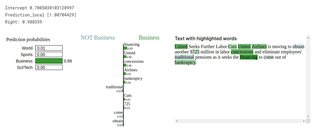
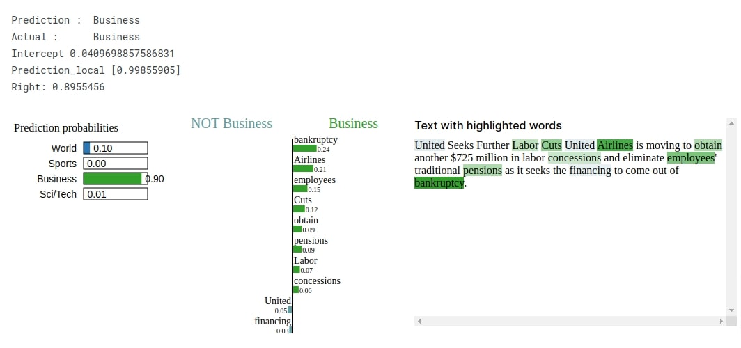
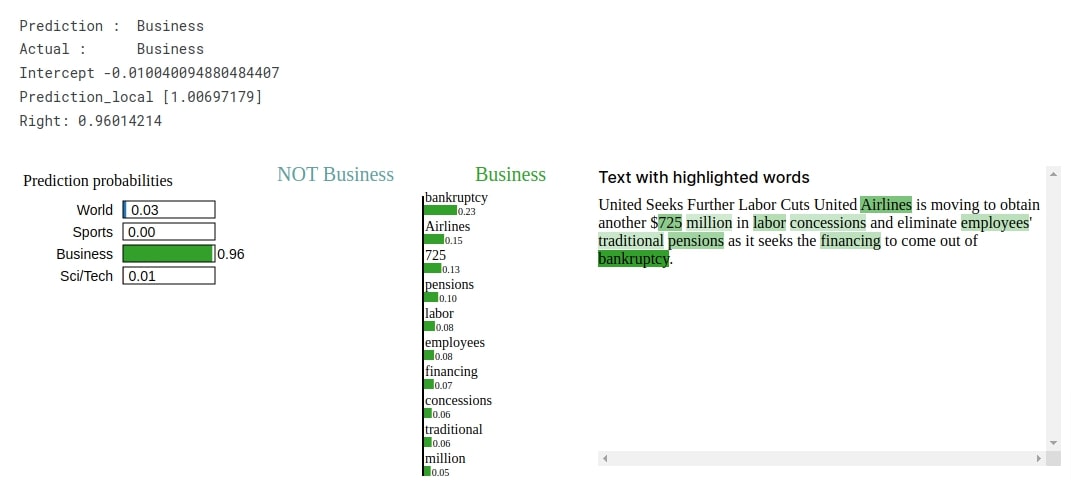
Below, we have called explain_instance() method with selected text example, helper function, and target label of text example. The method returned an Explanation object on which we have called show_in_notebook() method to generate visualization explaining prediction. We can notice from the visualization that words like 'financing', 'united', 'concessions', 'bankruptcy', 'cuts', etc are contributing to predicting the target label as Busines which makes sense as these are commonly used words in the business world.
explanation = explainer.explain_instance(X_test_text[idx], classifier_fn=make_predictions,
                                         labels=Y_test[idx:idx+1])
explanation.show_in_notebook()
Approach 2: Single LSTM Layer (Tokens Per Text Example=50, Embeddings Length=50, LSTM Output=75) 
Our approach in this section is almost the same as our approach in the previous section as it uses again single LSTM layer in the network. The only difference is in max tokens that we keep per text example. We have increased the number of tokens per text example to 50. The majority of the code in this section is the same as the previous section with only a change in max tokens per example.
Load Dataset And Create Data Loaders
Below, we have again loaded our datasets and created a data loader from it. This time, we have set max_words to 50 to keep the first 50 tokens per text example.
from torch.utils.data import DataLoader
from torchtext.data.functional import to_map_style_dataset

train_dataset, test_dataset  = torchtext.datasets.AG_NEWS()
train_dataset, test_dataset  = to_map_style_dataset(train_dataset), to_map_style_dataset(test_dataset)

target_classes = ["World", "Sports", "Business", "Sci/Tech"]

max_words = 50

train_loader = DataLoader(train_dataset, batch_size=1024, collate_fn=vectorize_batch, shuffle=True)
test_loader  = DataLoader(test_dataset , batch_size=1024, collate_fn=vectorize_batch)
for X, Y in train_loader:
    print(X.shape, Y.shape)
    break
Define LSTM Network
Below, we have defined our LSTM network which is exactly the same as our previous approach consisting of three layers (Embedding, LSTM, and Linear).
from torch import nn
from torch.nn import functional as F

embed_len = 50
hidden_dim = 75
n_layers=1

class LSTMClassifier(nn.Module):
    def __init__(self):
        super(LSTMClassifier, self).__init__()
        self.embedding_layer = nn.Embedding(num_embeddings=len(vocab), embedding_dim=embed_len)
        self.lstm = nn.LSTM(input_size=embed_len, hidden_size=hidden_dim, num_layers=n_layers, batch_first=True)
        self.linear = nn.Linear(hidden_dim, len(target_classes))

    def forward(self, X_batch):
        embeddings = self.embedding_layer(X_batch)
        hidden, carry = torch.randn(n_layers, len(X_batch), hidden_dim), torch.randn(n_layers, len(X_batch), hidden_dim)
        output, (hidden, carry) = self.lstm(embeddings, (hidden, carry))
        return self.linear(output[:,-1])
Train Network
Here, we have trained our network for 10 epochs and a learning rate of 0.001. The settings of training are the same as our previous approach. We'll be training all our networks using the same settings to make comparison easy. We can notice from the loss and accuracy getting printed after each epoch that our model seems to be doing a good job.
from torch.optim import Adam

epochs = 10
learning_rate = 1e-3

loss_fn = nn.CrossEntropyLoss()
lstm_classifier = LSTMClassifier()
optimizer = Adam(lstm_classifier.parameters(), lr=learning_rate)

TrainModel(lstm_classifier, loss_fn, optimizer, train_loader, test_loader, epochs)
Evaluate Network Performance
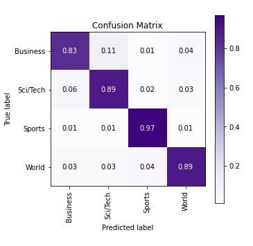
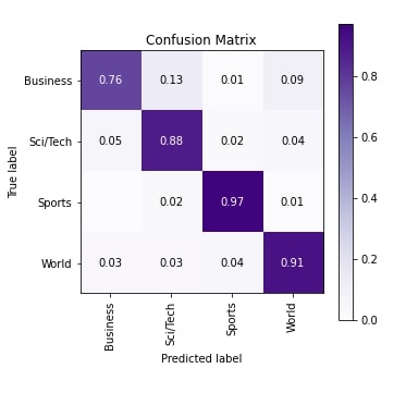
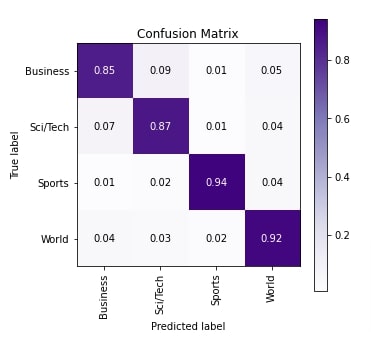
In this section, we have evaluated the performance of our network by calculating accuracy, classification report and confusion matrix metrics on test predictions. We can notice from the accuracy that it has improved a little bit compared to our previous approach. We can notice from the confusion matrix plot that our model is good at classifying text examples of categories Sci/Tech, Sports, and World compared to category Business.
from sklearn.metrics import accuracy_score, classification_report, confusion_matrix

Y_actual, Y_preds = MakePredictions(lstm_classifier, test_loader)

print("Test Accuracy : {}".format(accuracy_score(Y_actual, Y_preds)))
print("\nClassification Report : ")
print(classification_report(Y_actual, Y_preds, target_names=target_classes))
print("\nConfusion Matrix : ")
print(confusion_matrix(Y_actual, Y_preds))
from sklearn.metrics import confusion_matrix
import scikitplot as skplt
import matplotlib.pyplot as plt
import numpy as np

skplt.metrics.plot_confusion_matrix([target_classes[i] for i in Y_actual], [target_classes[i] for i in Y_preds],
                                    normalize=True,
                                    title="Confusion Matrix",
                                    cmap="Purples",
                                    hide_zeros=True,
                                    figsize=(5,5)
                                    );
plt.xticks(rotation=90);
Explain Predictions Using LIME Algorithm
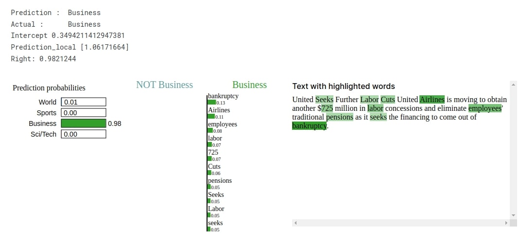
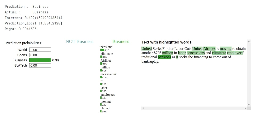
In this section, we have again tried to explain the prediction made by our trained model on the randomly selected text example from the test dataset using LIME algorithm. Our model has correctly predicted the target label as Business for randomly selected text example. From the visualization generated using lime, we can notice that words like 'bankruptcy', 'employees', 'airlines', 'cuts', 'pensions', 'labor', 'concessions', etc are contributing to predicting target label as Business.
from lime import lime_text
import numpy as np

explainer = lime_text.LimeTextExplainer(class_names=target_classes, verbose=True)

rng = np.random.RandomState(1)
idx = rng.randint(1, len(X_test_text))
X = [vocab(tokenizer(text)) for text in X_test_text[idx:idx+1]]
X = [tokens+([0]* (max_words-len(tokens))) if len(tokens)<max_words else tokens[:max_words] for tokens in X] ## Bringing all samples to max_words length.
preds = lstm_classifier(torch.tensor(X, dtype=torch.int32))
preds = F.softmax(preds, dim=-1)

print("Prediction : ", target_classes[preds.argmax()])
print("Actual :     ", target_classes[Y_test[idx]])

explanation = explainer.explain_instance(X_test_text[idx], classifier_fn=make_predictions,
                                         labels=Y_test[idx:idx+1])
explanation.show_in_notebook()
Approach 3: Multiple LSTM Layers (Tokens Per Text Example=50, Embeddings Length=50, LSTM Output=75) 
Till now, both approaches that we tried used a single LSTM layer. Our approach in this section uses 3 LSTM layers in sequence. We have tried this approach to check whether it further helps improve the performance of the network. The majority of the code is the same as our previous approaches with minor changes in network definition.
Define LSTM Network
Below, we have defined the network that we'll be using in this section. The network definition is exactly the same as our previous approaches with only a change in n_layers which is set to 3 to inform LSTM() constructor to create three LSTM layers.
As usual, after defining the network, we have initialized it and printed the shape of weights/biases of layers.
from torch import nn
from torch.nn import functional as F

embed_len = 50
hidden_dim = 75
n_layers=3

class LSTMClassifier(nn.Module):
    def __init__(self):
        super(LSTMClassifier, self).__init__()
        self.embedding_layer = nn.Embedding(num_embeddings=len(vocab), embedding_dim=embed_len)
        self.lstm = nn.LSTM(input_size=embed_len, hidden_size=hidden_dim, num_layers=n_layers, batch_first=True)
        self.linear = nn.Linear(hidden_dim, len(target_classes))

    def forward(self, X_batch):
        embeddings = self.embedding_layer(X_batch)
        hidden, carry = torch.randn(n_layers, len(X_batch), hidden_dim), torch.randn(n_layers, len(X_batch), hidden_dim)
        output, (hidden, carry) = self.lstm(embeddings, (hidden, carry))
        return self.linear(output[:,-1])
lstm_classifier = LSTMClassifier()

lstm_classifier
for layer in lstm_classifier.children():
    print("Layer : {}".format(layer))
    print("Parameters : ")
    for param in layer.parameters():
        print(param.shape)
    print()
Train Network
Below, we have trained our network using the same settings that we have been using for all our approaches till now. We can notice from the loss and accuracy getting printed after each epoch that the model is doing a good job at the text classification task.
from torch.optim import Adam

epochs = 10
learning_rate = 1e-3

loss_fn = nn.CrossEntropyLoss()
lstm_classifier = LSTMClassifier()
optimizer = Adam(lstm_classifier.parameters(), lr=learning_rate)

TrainModel(lstm_classifier, loss_fn, optimizer, train_loader, test_loader, epochs)
Evaluate Network Performance
In this section, we have evaluated the accuracy, classification report and confusion matrix metrics on test predictions. We can notice from the accuracy that it is almost the same as our accuracy from the previous section with not much improvement. When we look at the confusion matrix plot generated using scikit-plot, we can notice that the model has not good accuracy in all target categories.
from sklearn.metrics import accuracy_score, classification_report, confusion_matrix

Y_actual, Y_preds = MakePredictions(lstm_classifier, test_loader)

print("Test Accuracy : {}".format(accuracy_score(Y_actual, Y_preds)))
print("\nClassification Report : ")
print(classification_report(Y_actual, Y_preds, target_names=target_classes))
print("\nConfusion Matrix : ")
print(confusion_matrix(Y_actual, Y_preds))
from sklearn.metrics import confusion_matrix
import scikitplot as skplt
import matplotlib.pyplot as plt
import numpy as np

skplt.metrics.plot_confusion_matrix([target_classes[i] for i in Y_actual], [target_classes[i] for i in Y_preds],
                                    normalize=True,
                                    title="Confusion Matrix",
                                    cmap="Purples",
                                    hide_zeros=True,
                                    figsize=(5,5)
                                    );
plt.xticks(rotation=90);
Explain Predictions Using LIME Algorithm
In this section, we have again explained the prediction made by our trained network on a randomly selected test example using LIME algorithm. Our network correctly predicts the target label as Business for the selected text example. The visualization shows that words like 'bankruptcy', 'employees', 'airlines', 'labor', 'cuts', 'pensions', etc are contributing to predicting target label as Business which makes sense.
from lime import lime_text
import numpy as np

explainer = lime_text.LimeTextExplainer(class_names=target_classes, verbose=True)

rng = np.random.RandomState(1)
idx = rng.randint(1, len(X_test_text))
X = [vocab(tokenizer(text)) for text in X_test_text[idx:idx+1]]
X = [tokens+([0]* (max_words-len(tokens))) if len(tokens)<max_words else tokens[:max_words] for tokens in X] ## Bringing all samples to max_words length.
preds = lstm_classifier(torch.tensor(X, dtype=torch.int32))
preds = F.softmax(preds, dim=-1)

print("Prediction : ", target_classes[preds.argmax()])
print("Actual :     ", target_classes[Y_test[idx]])

explanation = explainer.explain_instance(X_test_text[idx], classifier_fn=make_predictions,
                                         labels=Y_test[idx:idx+1])
explanation.show_in_notebook()
Approach 4: Stacking Multiple LSTM Layers (Tokens Per Text Example=50, Embeddings Length=50, LSTM Output=75) 
Our approach in this section again tries to use multiple LSTM layers in the network but this time, the output shape of each LSTM layer is different, unlike our previous approach where it was the same for all 3 LSTM layers. The only change in the code in this section is in the definition of network, the rest of the code is exactly the same as our previous approaches.
Define LSTM Network
Below, we have defined the network that we'll be using for our task in this section. We have defined three LSTM layers this time with different hidden_size this time (50, 60, and 75). The output of the embedding layer is given to the first LSTM whose output is given to the second LSTM layer. The output of the second LSTM layer is given to the third LSTM and the output of the last LSTM layer is given to the Linear layer. Please make a NOTE that we have defined hidden and carry for each LSTM layer separately.
After defining the network, we initialized it and printed the shape of weights/biases of layers.
from torch import nn
from torch.nn import functional as F

embed_len = 50
hidden_dim1 = 50
hidden_dim2 = 60
hidden_dim3 = 75
n_layers=1

class LSTMClassifier(nn.Module):
    def __init__(self):
        super(LSTMClassifier, self).__init__()
        self.embedding_layer = nn.Embedding(num_embeddings=len(vocab), embedding_dim=embed_len)
        self.lstm1 = nn.LSTM(input_size=embed_len, hidden_size=hidden_dim1, num_layers=1, batch_first=True)
        self.lstm2 = nn.LSTM(input_size=hidden_dim1, hidden_size=hidden_dim2, num_layers=1, batch_first=True)
        self.lstm3 = nn.LSTM(input_size=hidden_dim2, hidden_size=hidden_dim3, num_layers=1, batch_first=True)
        self.linear = nn.Linear(hidden_dim3, len(target_classes))

    def forward(self, X_batch):
        embeddings = self.embedding_layer(X_batch)
        hidden, carry = torch.randn(n_layers, len(X_batch), hidden_dim1), torch.randn(n_layers, len(X_batch), hidden_dim1)
        output, (hidden, carry) = self.lstm1(embeddings, (hidden, carry))

        hidden, carry = torch.randn(n_layers, len(X_batch), hidden_dim2), torch.randn(n_layers, len(X_batch), hidden_dim2)
        output, (hidden, carry) = self.lstm2(output, (hidden, carry))

        hidden, carry = torch.randn(n_layers, len(X_batch), hidden_dim3), torch.randn(n_layers, len(X_batch), hidden_dim3)
        output, (hidden, carry) = self.lstm3(output, (hidden, carry))
        return self.linear(output[:,-1])
lstm_classifier = LSTMClassifier()

lstm_classifier
for layer in lstm_classifier.children():
    print("Layer : {}".format(layer))
    print("Parameters : ")
    for param in layer.parameters():
        print(param.shape)
    print()
Train Network
Below, we have trained our network using the same settings that we have been using for all our approaches. We can notice from the loss and accuracy that our model is doing a good job.
from torch.optim import Adam

epochs = 10
learning_rate = 1e-3

loss_fn = nn.CrossEntropyLoss()
lstm_classifier = LSTMClassifier()
optimizer = Adam(lstm_classifier.parameters(), lr=learning_rate)

TrainModel(lstm_classifier, loss_fn, optimizer, train_loader, test_loader, epochs)
Evaluate Network Performance
Below, we have evaluated the performance of our trained network by calculating accuracy, classification report and confusion matrix metrics on test predictions. We can notice from the accuracy that our model has the least accuracy of all approaches, we tried till now. The confusion matrix plot shows that model is doing a good job at classifying text documents of categories Sci/Tech, Sports, and World compared to category Business.
from sklearn.metrics import accuracy_score, classification_report, confusion_matrix

Y_actual, Y_preds = MakePredictions(lstm_classifier, test_loader)

print("Test Accuracy : {}".format(accuracy_score(Y_actual, Y_preds)))
print("\nClassification Report : ")
print(classification_report(Y_actual, Y_preds, target_names=target_classes))
print("\nConfusion Matrix : ")
print(confusion_matrix(Y_actual, Y_preds))
from sklearn.metrics import confusion_matrix
import scikitplot as skplt
import matplotlib.pyplot as plt
import numpy as np

skplt.metrics.plot_confusion_matrix([target_classes[i] for i in Y_actual], [target_classes[i] for i in Y_preds],
                                    normalize=True,
                                    title="Confusion Matrix",
                                    cmap="Purples",
                                    hide_zeros=True,
                                    figsize=(5,5)
                                    );
plt.xticks(rotation=90);
Explain Predictions Using LIME Algorithm
In this section, we have again explained the prediction made by our network on a randomly selected test example using LIME algorithm. The network correctly predicts the target category as Business for the selected sample. The visualization shows that words like 'bankruptcy', 'airlines', 'pensions', 'pensions', 'labor', 'employees', 'financing', 'concessions', etc are contributing to predicting target category as Business.
from lime import lime_text
import numpy as np

explainer = lime_text.LimeTextExplainer(class_names=target_classes, verbose=True)

rng = np.random.RandomState(1)
idx = rng.randint(1, len(X_test_text))
X = [vocab(tokenizer(text)) for text in X_test_text[idx:idx+1]]
X = [tokens+([0]* (max_words-len(tokens))) if len(tokens)<max_words else tokens[:max_words] for tokens in X] ## Bringing all samples to max_words length.
preds = lstm_classifier(torch.tensor(X, dtype=torch.int32))
preds = F.softmax(preds, dim=-1)

print("Prediction : ", target_classes[preds.argmax()])
print("Actual :     ", target_classes[Y_test[idx]])

explanation = explainer.explain_instance(X_test_text[idx], classifier_fn=make_predictions,
                                         labels=Y_test[idx:idx+1])
explanation.show_in_notebook()
Approach 5: Multiple Bidirectional LSTM Layers (Tokens Per Text Example=50, Embeddings Length=50, LSTM Output=75) 
Our approach in this section has the same network definition as our third approach. We have again used a network with 3 LSTM layers but this time, we have kept all LSTM layers bidirectional. As we had said earlier, the LSTM layer goes through each token of the text example generating output that it uses for the calculation of the next token in the same text example. This process of going through all tokens of text examples happens only in one direction (forward) in the normal LSTM layer. But in the case of the bidirectional LSTM layer, it goes through text tokens of text example in both forward and backward directions. It tries to capture some pattern if present in the backward direction as well.
Define LSTM Network
Our network definition in this section is exactly the same as our network definition from the third approach with minor changes. We have set bidirectional parameter to True in LSTM() constructor to inform it to create bidirectional LSTM layers. The input units of Linear layer are 2 times the output size of the LSTM layer because the now output of the LSTM layer contains combine output generated in both directions (forward and backward).
After defining the network, we initialized it and printed the shape of weights/biases of each layer of the network.
from torch import nn
from torch.nn import functional as F

embed_len = 50
hidden_dim = 75
n_layers=3

class LSTMClassifier(nn.Module):
    def __init__(self):
        super(LSTMClassifier, self).__init__()
        self.embedding_layer = nn.Embedding(num_embeddings=len(vocab), embedding_dim=embed_len)
        self.lstm = nn.LSTM(input_size=embed_len, hidden_size=hidden_dim, num_layers=n_layers, batch_first=True,
                            bidirectional=True)
        self.linear = nn.Linear(2*hidden_dim, len(target_classes))  ## Input dimension are 2 times hidden dimensions due to bidirectional results

    def forward(self, X_batch):
        embeddings = self.embedding_layer(X_batch)
        hidden, carry = torch.randn(2*n_layers, len(X_batch), hidden_dim), torch.randn(2*n_layers, len(X_batch), hidden_dim)
        output, (hidden, carry) = self.lstm(embeddings, (hidden, carry))
        return self.linear(output[:,-1])
lstm_classifier = LSTMClassifier()

lstm_classifier
for layer in lstm_classifier.children():
    print("Layer : {}".format(layer))
    print("Parameters : ")
    for param in layer.parameters():
        print(param.shape)
    print()
Train Network
Below, we have trained our network using the same settings that we have been using for all our approaches. We can notice from the loss and accuracy values getting printed after each epoch that our model is doing a good job.
from torch.optim import Adam

epochs = 10
learning_rate = 1e-3

loss_fn = nn.CrossEntropyLoss()
lstm_classifier = LSTMClassifier()
optimizer = Adam(lstm_classifier.parameters(), lr=learning_rate)

TrainModel(lstm_classifier, loss_fn, optimizer, train_loader, test_loader, epochs)
Evaluate Network Performance
In this section, we have evaluated the performance of the network as usual by calculating accuracy, classification report and confusion matrix metrics on test predictions. We can notice from the accuracy that the model has the almost same accuracy as our model from the second approach. The network seems to be doing good for all target categories from the confusion matrix plot.
from sklearn.metrics import accuracy_score, classification_report, confusion_matrix

Y_actual, Y_preds = MakePredictions(lstm_classifier, test_loader)

print("Test Accuracy : {}".format(accuracy_score(Y_actual, Y_preds)))
print("\nClassification Report : ")
print(classification_report(Y_actual, Y_preds, target_names=target_classes))
print("\nConfusion Matrix : ")
print(confusion_matrix(Y_actual, Y_preds))
from sklearn.metrics import confusion_matrix
import scikitplot as skplt
import matplotlib.pyplot as plt
import numpy as np

skplt.metrics.plot_confusion_matrix([target_classes[i] for i in Y_actual], [target_classes[i] for i in Y_preds],
                                    normalize=True,
                                    title="Confusion Matrix",
                                    cmap="Purples",
                                    hide_zeros=True,
                                    figsize=(5,5)
                                    );
plt.xticks(rotation=90);
Explain Predictions Using LIME Algorithm
In this section, we have explained the prediction made by our trained network on a randomly selected test example using LIME algorithm. The network correctly predicts the target label as Business for the selected text example. The words like 'pensions', 'million', 'concessions', 'labor', 'employees', etc are contributing to predicting target label as Business.
from lime import lime_text
import numpy as np

explainer = lime_text.LimeTextExplainer(class_names=target_classes, verbose=True)

rng = np.random.RandomState(1)
idx = rng.randint(1, len(X_test_text))
X = [vocab(tokenizer(text)) for text in X_test_text[idx:idx+1]]
X = [tokens+([0]* (max_words-len(tokens))) if len(tokens)<max_words else tokens[:max_words] for tokens in X] ## Bringing all samples to max_words length.
preds = lstm_classifier(torch.tensor(X, dtype=torch.int32))
preds = F.softmax(preds, dim=-1)

print("Prediction : ", target_classes[preds.argmax()])
print("Actual :     ", target_classes[Y_test[idx]])

explanation = explainer.explain_instance(X_test_text[idx], classifier_fn=make_predictions,
                                         labels=Y_test[idx:idx+1])
explanation.show_in_notebook()
7. Results Summary and Further Recommendations
The below table highlights the settings and performance of different network approaches that we tried.
| Approach | Max Tokens | Embedding Length | LSTM Hidden Dimension | Test Accuracy (%) |
|---|---|---|---|---|
| Single LSTM Layer | 25 | 50 | 75 | 88.26 |
| Single LSTM Layer | 50 | 50 | 75 | 89.57 |
| Multiple LSTM Layers (3 Layers) | 50 | 50 | 75 | 89.51 |
| Stacking Multiple LSTM Layers (3 Layers) | 50 | 50 | 50,60,75 | 88.03 |
| Multiple Bidirectional LSTM Layers (3 Layers) | 50 | 50 | 75 | 89.56 |
Further Suggestions
Below, we have listed a few suggestions that can be tried to further improve network accuracy.
- Try different tokens per text example.
- Try different word embedding lengths.
- Try different LSTM hidden sizes.
- Add a few more linear/dense layers after LSTM layers.
- Stack more LSTM layers.
- Try different weight initialization techniques.
- Try learning rate scheduling.
- Train network for more epochs.
This ends our small tutorial explaining how we can create a neural network with LSTM layers using PyTorch and use it for text classification tasks. Please feel free to let us know your views in the comments section.
References
 Sunny Solanki
Sunny Solanki
Intro: Software Developer | Youtuber | Bonsai Enthusiast
About: Sunny Solanki holds a bachelor's degree in Information Technology (2006-2010) from L.D. College of Engineering. Post completion of his graduation, he has 8.5+ years of experience (2011-2019) in the IT Industry (TCS). His IT experience involves working on Python & Java Projects with US/Canada banking clients. Since 2020, he’s primarily concentrating on growing CoderzColumn.
His main areas of interest are AI, Machine Learning, Data Visualization, and Concurrent Programming. He has good hands-on with Python and its ecosystem libraries.
Apart from his tech life, he prefers reading biographies and autobiographies. And yes, he spends his leisure time taking care of his plants and a few pre-Bonsai trees.
Contact: sunny.2309@yahoo.in


![YouTube Subscribe]() Comfortable Learning through Video Tutorials?
Comfortable Learning through Video Tutorials?
If you are more comfortable learning through video tutorials then we would recommend that you subscribe to our YouTube channel.
![Need Help]() Stuck Somewhere? Need Help with Coding? Have Doubts About the Topic/Code?
Stuck Somewhere? Need Help with Coding? Have Doubts About the Topic/Code?
 Stuck Somewhere? Need Help with Coding? Have Doubts About the Topic/Code?
When going through coding examples, it's quite common to have doubts and errors.
If you have doubts about some code examples or are stuck somewhere when trying our code, send us an email at coderzcolumn07@gmail.com. We'll help you or point you in the direction where you can find a solution to your problem.
You can even send us a mail if you are trying something new and need guidance regarding coding. We'll try to respond as soon as possible.
![Share Views]() Want to Share Your Views? Have Any Suggestions?
Want to Share Your Views? Have Any Suggestions?
 Want to Share Your Views? Have Any Suggestions?
If you want to
- provide some suggestions on topic
- share your views
- include some details in tutorial
- suggest some new topics on which we should create tutorials/blogs
 pytorch, LSTM, text-classification, word-embeddings