How to Use LIME to Interpret Predictions of ML Models?¶

Explaining or Interpreting the predictions of machine learning models has become of prime importance nowadays as we work with complicated deep networks that handle unstructured data types like image, audio, text, etc, and structured data with thousands of features.

Why Interpret Predictions of ML Model?¶

The traditional ML metrics like accuracy, confusion matrix, classification report, r2 score, ROC AUC curves, precision-recall curves, etc does not give machine learning practitioner enough confidence about model performance as well as reliability. We can have machine learning models that give more than 95% accuracy but fails to recognize some classes of dataset due to use of irrelevant features during prediction (E.g., Cat vs Dog classifier can be utilizing background pixels to recognize an object in an image rather than actual cat/dog object pixels).

Model Architecture and Interpretability Relationship¶

Model architecture and interpretability generally have an inverse relationship. The more complicated the model the less interpretable it is. Models like deep neural networks (Generated using Keras, PyTorch, TensorFlow, sklearn, etc), gradient boosting machines, and random forests give high accuracy but are less interpretable compared to models like linear regression & logistic regression (Generated using sklearn, statsmodels) which might give less accuracy but are easy to interpret.

Due to this, the deep neural networks are commonly referred to as black-box models whereas interpretable models like linear regression are referred to as white-box models.

It has become a need of the hour to better understand how features are contributing so that we can better understand models that make sense to persons who are not ML practitioners.

Which Python Libraries to Use for Interpreting ML Model Predictions?¶

Python has many libraries like lime, SHAP, eli5, captum, interpret, etc that provides different algorithms to explain predictions made by complex black-box as well as white-box models. We'll be primarily concentrating on lime today.

What Can You Learn From This Article?¶

As a part of this tutorial, we have explained how to use Python library lime to explain predictions made by ML models. It implements the famous LIME (Local Interpretable Model-Agnostic Explanations) algorithm and lets us create visualizations showing individual features contributions. Tutorial uses lime to explain predictions made by simple sklearn models trained on toy datasets. It covers in detail how we can use lime with structured datasets (tabular) and unstructured datasets (image & text). Both regression and classification models are covered.

The tutorial is a good starting point for someone who is new to lime. It explains the usage with simple models which makes it easy to grasp the API of library.

What is LIME (Local Interpretable Model-Agnostic Explanations)?¶

LIME algorithm stands for local interpretable model agnostic explanations that take any machine learning models as input and generates explanations about features contributions in making a prediction on an individual example. It assumes that the model is a black box model which means that it does not know the inner workings of models and generates an explanation based on this assumption. It let us generates an explanation for individual data example. The interpretation results of one example can be different than others.

If you are someone who wants to use lime for deep neural networks then we would recommend you to look at our References section at the end of tutorial. There we have listed tutorials that use lime on deep neural networks.

Below, we have listed important sections of tutorial to give an overview of the material covered.

Important Sections Of Tutorial¶

1. How LIME Works Internally?
2. Steps to Use "lime" to Explain Prediction
3. Important Sub-Modules Of "lime"
4. "lime_tabular": LIME For Structured Data ("Tabular")
   • 4.1. Regression
     • Load Dataset
     • Divide into Train/Test Sets
     • Train ML Model
     • Evaluate Network Performance using Traditional ML Metrics
     • Explain Individual Prediction using "LimeTabularExplainer"
   • 4.2. Binary Classification
   • 4.3. Multi-Class Classification
5. "lime_text": LIME For Unstructured Data ("Text")
   • 5.1. Text Classification
     • Load Data and Train Model
     • Explain Individual Prediction using "LimeTextExplainer"
6. "lime_image": LIME For Unstructured Data ("Image")
   • 6.1. Digits Multi-Class Image Classification
     • Load Data and Train Model
     • Explain Individual Prediction using "LimeImageExplainer"

1. How LIME Works Internally? ¶

Please feel free to skip this theoretical section if you are in hurry and want to get started with coding part.¶

Below we have tried to explain how LIME works internally. The steps are taken from a presentation given by Kasia Kulma (Ph.D.) on LIME and the link to the presentation is given in the references section last.

1. LIME takes an individual sample and generates a fake dataset based on it. It then permutes the fake dataset.
2. It then calculates distance metrics (or similarity metrics) between permuted fake data and original observations. This helps to understand how similar permuted fake data is compared to original data. The lime library methods provide us with options to try different similarity metrics for this purpose.
3. It then makes a prediction on this new permuted fake data using our original complex model.
4. It then picks features that best describe our complex model's performance on permuted fake data. The lime library lets us provide how many features to pick up.
5. It then fits simple model (like linear or logistic regression) on the combination of permuted fake data with selected m features and similarity scores computed in earlier steps. The lime library lets us provide a simple model that we want to use. Generally, it's linear regression or logistic regression but we can change it.
6. It then uses weights derived from that simple model for each feature to explain how each feature contributed to making a prediction for that sample when predicted using an original complex model.

Basically, it generates fake data using our input data, trains a simple ML model (one fake data) that has same performance as our complex black-box model, and uses this model's weights to describe features' importance.

2. Steps to Use "lime" to Explain Prediction ¶

1. Train ML Model
2. Create Explainer Object.
3. Call 'explain_instance()' method on Explainer Object. It'll return an Explanation object. This object has information about data features' importance.
   • We need to give an individual example (X[i]) and our trained ML model to this method that returns prediction. For classification tasks, it should return probabilities for all target categories.
   • We can also give a function to it that returns prediction/probabilities.
4. Call 'show_in_notebook()' method on Explanation Object. This will create a figure showing which features contributed to prediction.
   • Other methods can be used to retrieve feature importances in different formats.
     • 'as_list()'
     • 'as_map()'
     • 'as_html()'
     • 'as_pyplot_figure()'

3. Important Sub-Modules Of "lime" ¶

The lime has three main modules which can be used with different types of datasets. All these modules provide different types of Explainer objects for creating explanations:

1. "lime_tabular" - This sub-module is used for generating explanations for structured datasets (tables).
2. "lime_text" - Its used for generating explanations for text datasets.
3. "lime_image" - It's used for generating explanations for image datasets.

4. "lime_tabular": LIME For Structured Data ("Tabular") ¶

The lime has a module named lime_tabular which provides methods that can be used to generate explanations of the model which are trained on structured datasets. We'll be trying regression and classification models on different datasets and then use lime to generate explanations for random examples of the dataset.

We'll start by importing the necessary libraries.

4.1. Regression ¶

In this section, we have tried to solve a simple regression task involving Boston housing dataset. The task trains a simple ML model on dataset to predict housing prices. Then, we explain network prediction on individual examples using lime.

4.1.1 Load Dataset¶

As a part of the first example, we'll be using the Boston housing dataset available from scikit-learn. It has information about various houses sold in Boston in past and we'll be predicting the median value of a home in 1000's dollars.

First, We have loaded the dataset from the sklearn and printed a description of the dataset. Then, we loaded the dataset as a pandas dataframe to display the first few samples of data.

4.1.2 Divide Dataset into Train/Test Sets¶

Below we have divided the original dataset into the train (90%) and test (10%) sets.

4.1.3 Train Model and Calculate ML Metrics¶

We have now fitted a linear regression model from scikit-learn on train dataset and then evaluated r2 score of the trained model on test & train predictions. Next, we'll explain the prediction made by network using lime.

If you are interested in learning about various ML metrics available from sklearn then we would recommend you below link. Please feel free to check it in your free time. It covers majority of metrics.

• Model Evaluation Metrics in Scikit-Learn

4.1.4 Explain Individual Prediction using "LimeTabularExplainer"¶

As this is a structured dataset problem, we'll be using 'LimeTabularExplainer' available from 'lime_tabular' for explaining prediction. We have covered step by step guide to explain predictions with various useful methods.

1. Create Explainer Object¶

The lime_tabular module has a class named LimeTabularExplainer which takes as input train data and generates an explainer object which can then be used to explain individual prediction.

Below is a list of important parameters of the LimeTabularExplainer class.

• training_data - It accepts samples (numpy 2D array) that were used to train the model.
• mode - It accepts one of the below strings
  • 'classification' - Default Value
  • 'regression'
• training_labels - It accepts a list of training labels.
• feature_names - It accepts a list of feature names of data.
• categorical_features - It accepts list of indices (e.g - [1,4,5,6]) in training data which represents categorical features.
• categorical_names - It accepts mapping (dict) from integer to list of names. The mapping will have information about all possible values in a particular categorical column. The categorical_names[x][y] will be pointing to yth value of column with index x in dataset.
• class_names - It accepts a list of class names for the classification tasks.
• feature_selection - It accepts a string value from below list for feature selection when selecting the m-best feature as described in the internal working of LIME earlier.
  • 'forward_selection'
  • 'lasso_path'
  • 'none'
  • 'auto'
• random_state - It accepts integer or np.RandomState object specifying random state so that we can reproduce the same results each time we rerun the process.

Below we are creating the LimeTabularExplainer object by passing it train data, mode as regression, and feature names.

2. Create Explanation object using "explain_instance()"¶

The LimeTabularExplainer instance has a method named explain_instance() which takes single data example and ML-model/function as input. It returns an Explanation object. This Explanation object has information about features contributions to this particular prediction.

The input ML-model/function is used for prediction. In majority of cases, we can provide our ML model as it is to explain_instance() but there can be cases where we are performing pre-processing steps on input data before giving it to network for prediction (E.g., pre-processing text data). In those cases, we can give a function that takes an example as input and returns prediction.

Here is a list of important parameters of the explain_instance() method:

• data_row - It accepts 1 data sample represented as 1d numpy array or script sparse matrix as input.
• predict_fn - It accepts prediction function which takes as input sample passed to data_row as input and generates an actual prediction for regression tasks and class probabilities for classification tasks.
• labels - It takes as input a list of class labels to explain the multi-class classification tasks.
• top_labels - It takes as input integer specifying top k class with highest probabilities from prediction to be displayed.
• num_features - It accepts integer numbers specifying top k features to keep in explanation. The default is 10.
• num_samples - It accepts integers specifying the size of samples to use for training a simple linear model. The default is 5000.
• distance_metric - It accepts distance metric to use to compute the similarity between original and permuted samples. The default value is the string euclidean.
• model_regressor - It accepts a simple model which should be used to train permuted data with m best features. The default is ridge regression from sklearn.

Below we are passing a random sample taken from the test dataset and reference to predict the method of the linear regression model as input to the method and it returns Explanation object.

3. Visualize Features Importances using "show_in_notebook()"¶

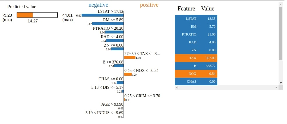
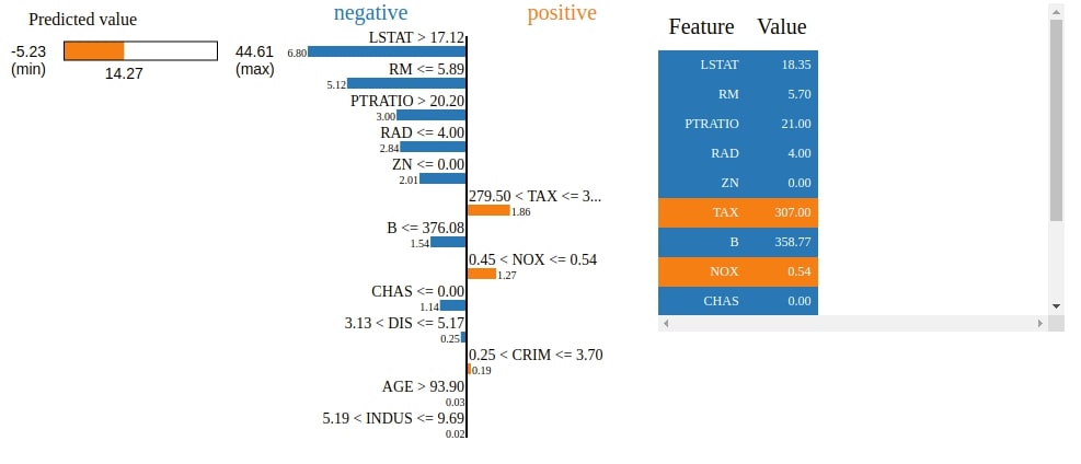
The Explainer object has a method named show_in_notebook() which will explain how we come to a particular prediction based on feature contribution as HTML. It'll create a visualization showing feature contributions.

We can notice that visualization has a progress bar, bar chart, and table. The progress bar shows range in which value varies and actual prediction. The bar chart shows features that contributed positively and negatively to prediction. The table shows features contributions.

Below the HTML figure shows us the actual predicted value, a bar chart showing weights of how features contributed to this prediction, and a table showing actual feature values.

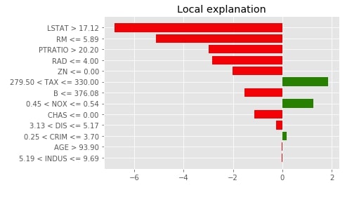
4. Visualize Feature Importances using "as_pyplot_figure()"¶

Below we have called the as_pyplot_figure() method to generate a bar chart of feature contribution for this sample.

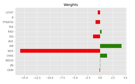
Below we have printed actual global weights we got from the linear regression model as a matplotlib bar chart.

5. Retrieve Features Importances as List using "as_list()"¶

Below we are calling the as_list() method on the Explanation object which returns explanation as a list of tuples where the first value of tuple is condition and the second value contribution of the feature value based on condition.

6. Retrieve Features Importances as Dictionary using "as_map()"¶

Below we have called the as_map() method which is exactly the same as the as_list() method for regression but useful for classification tasks because it'll return a dictionary where the key is each class of task and value is a list of feature index and their contribution in predicting that class.

7. Retrieve Features Importances as HTML using "as_html()"¶

The explanation object has another method named as_html() which returns explanation as HTML stored in a string. We can pass this string to IPython's HTML method for generating HTML output.

Jupyter notebook let us visualize rich contents of different types. Please feel free to check below link in your free time to learn about it.

• Display Rich Contents (Audio, Video, Image, HTML, etc) in Jupyter Notebook

8. Retrieve Average Local and Global Prediction Value¶

Below we have printed local prediction and global prediction using explanation. The local prediction is generated by a simple model that was trained on a combination of m best feature permuted data and similarity scores data. We can see that it's quite close to the actual prediction using our complex model.

9. Save Features Importances to HTML using "save_to_file()"¶

We can save explanation as HTML file by calling save_to_file() method on explanation.

Once we have saved a file as HTML then we can read it and display contents like we earlier did in as_html() section using IPython module.

4.2. Binary Classification ¶

The second example that we'll use for explaining the usage of 'lime_tabular' is a binary classification problem. We'll be using a breast cancer dataset available from scikit-learn for this purpose. The dataset has measurements of tumor size as data features and target variable is binary telling us whether a tumor is benign (1) or malignant (0).

4.2.1 Load Dataset, Train Model and Calculate ML Metrics¶

Below, We have loaded breast cancer dataset from sklearn and then printed a description of the dataset which explains individual features of the dataset.

After loading dataset, we divided it into the train (90%) and test (10%) sets, fitted logistic regression on train data, and evaluated metrics like accuracy, confusion matrix, and classification report on the test dataset. We can notice from the results that our model seems to be doing a good job at binary classification task.

• Model Evaluation Metrics in Scikit-Learn

4.2.2 Explain Individual Prediction using "LimeTabularExplainer"¶

Now, we'll explain individual prediction using 'lime'.

1. Create Explainer Object¶

Below we have created a LimeTabularExplainer object based on the training dataset. We'll be using this explainer object to explain a random sample from the test dataset.

2. Create Explanation Object and Visualize Feature Importances¶

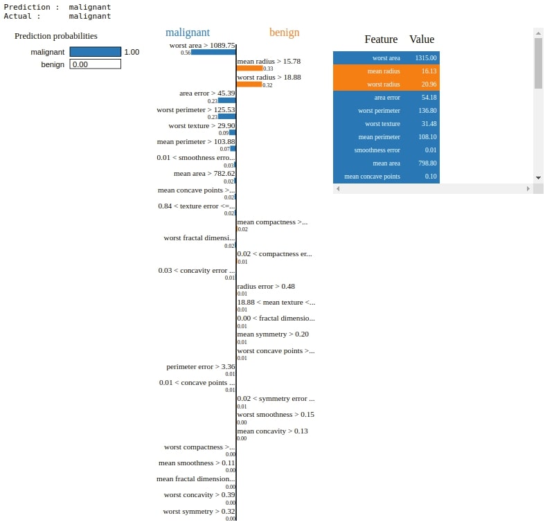
Below we have taken a random example from the test dataset. We have then called the explain_instance() method on explainer object passing it selected random example and reference to predict_proba() method of logistic regression to generate an explanation object for this random sample. We have then called show_in_notebook() method on explanation object to generate HTML of explanation.

The HTML shows prediction, a bar chart of the contribution of features, and a table with actual feature values. The bar chart is sorted from the most important features to the least important. We can pass a number of important features we want to see to the num_features parameter of the explain_instance() method.

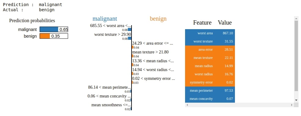
3. Visualize Features Importances for Wrong Predictions¶

Below we are explaining another random sample from the test dataset for which the model makes the wrong prediction. We are retrieving indices of samples from test data for which model is making mistake. We are then randomly selecting one index from it. We then pass the sample with that index to the explain_instance() method to generate an explanation object. Please make a note that we are only displaying the top 10 features which contribute most to prediction.

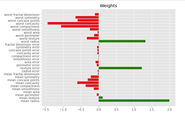
4. Visualizing Global Features Importances from LIME ML Model Weights¶

Below we have plotted a bar chart of global feature importance based on weights derived from logistic regression. We can use it to compare it with the bar chart generated for individual data samples.

4.3. Multi-Class Classification ¶

As a part of our third example for demonstrating usage of the 'lime_tabular' module, we'll be using a multi-class classification problem.

NOTE: Please feel free to skip this section if you have understood lime usage for classification from previous example. You can continue from next sections which covers usage with "text" and "image" datasets.¶

4.3.1 Load Dataset, Train Model and Calculate ML Metrics¶

Below, we have loaded a wine dataset available from sklearn which has information about various ingredients used in three different types of wine.

After loading it, we have divided data into train/test sets, trained GradientBoostingClassifier on train data, and printed metrics like accuracy, confusion matrix, and classification report on the test dataset.

We can notice from the results that our model seems to be doing a good job at multi-class classification task.

4.3.2 Explain Individual Prediction using "LimeTabularExplainer"¶

1. Create Explainer Instance¶

Below we have generation LimeTabularExplainer based on train data.

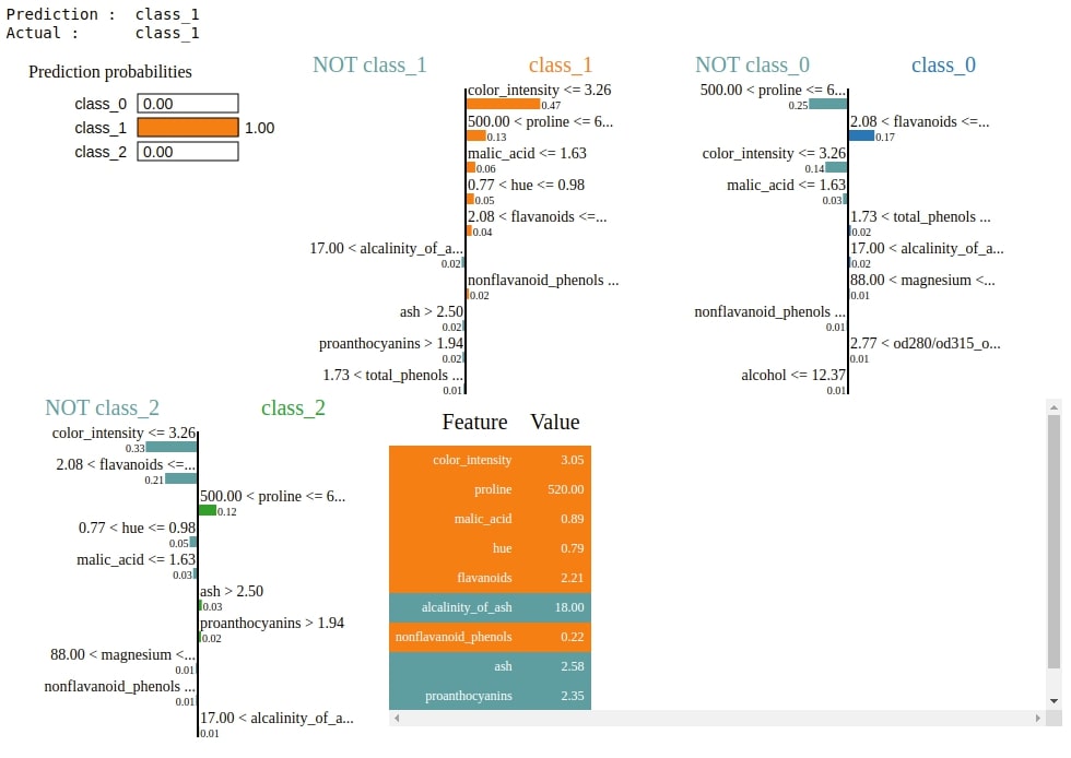
2. Explain Correct Predictions¶

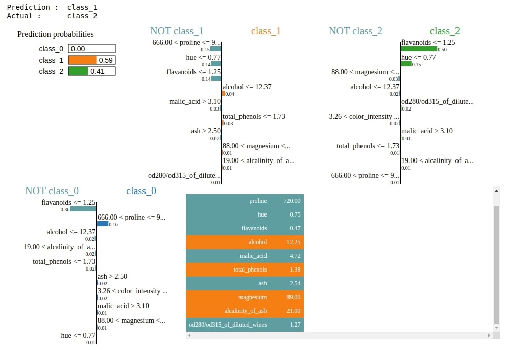
Below we are explaining a random sample from test data using an explanation object. We can see that this time we see three different bar charts showing features contributions, one for each class.

If we want to see bar charts of particular classes only then we can pass class names as a list to the labels parameter of the explain_instance() method. We can also pass an integer to the top_labels method and it'll show that many top classes have a high probability in model prediction.

3. Explain Incorrect Predictions¶

Below we are plotting an explanation for a random sample from test data for which model prediction is going wrong.

5. "lime_text": LIME For Unstructured Data ("Text") ¶

The 'lime_text' module of lime provides explainers that can help us explain unstructured text data. We'll be explaining how to use the text explainer available in the 'lime_text' module of lime as a part of this section.

5.1. Text Classification¶

The first example that we'll use for explaining the usage of the 'lime_text' module is a binary classification problem. We'll be using the spam/ham messages dataset available from UCI to classify whether text data present in the mail is spam or not.

5.1.1 Load Dataset¶

We'll first download data from the UCI ML data directory and then will perform classification by reading a file.

Below we have written a simple code that reads one line of data from the SMSSpamCollection text file and retrieves mail content. We have also later counted a number of spam and ham mails.

5.1.2 Divide Dataset into Train and Test Sets¶

We have then divided the dataset into the train (75%) and test (25%) sets.

5.1.3 Vectorize Datasets, Train Model and Calculate ML Metrics¶

Below we have first transformed text data from text to float format using TF-IDF vectorizer and then fitted that transformed data to a random forest classifier.

After completing training, we evaluated model performance on test dataset by evaluating classification metrics like accuracy, confusion matrix, and classification report.

If you are interested in learning about feature extraction from text data which we have performed here then please feel free to check our tutorial on the same which gives details insight on the topic.

• Feature Extraction from Text Data using Scikit-Learn

5.1.4 Explain Individual Prediction using "LimeTextExplainer"¶

Now, we'll explain predictions on text data using "lime".

1. Create "LimeTextExplainer" Object¶

The LimeTextExplainer class of the lime_text module provides functionality to handle unstructured text data and generate an explanation for it. Below we have first created the LimeTextExplainer object.

Here we have given a list of important parameters of LimeTextExplainer which one can tweak according to their need.

• class_names - It accepts a list of class names as input.
• feature_selection - It accepts a string value from below list for feature selection when selecting the m-best feature as described in the internal working of LIME earlier.
  • 'forward_selection'
  • 'lasso_path'
  • 'none'
  • 'auto'
• split_expression - It accepts the regular expression of a function. The regular expression will be responsible for generating tokens.
• random_state - It accepts integer or np.RandomState object specifying random state so that we can reproduce the same results each time we rerun the process.

Please make a NOTE that there are a few other parameters that we have not mentioned here but can be useful to someone with different scenarios.

Below we have created a LimeTextExplainer object with class names passed to it.

2. Define Prediction Function¶

Below, we have created a function that takes as input single sample of text data as input and then returns a prediction informing text is spam or ham.

As a part of the function, we are first transforming text using the TF-IDF vectorizer and then returning probabilities for it using random forest. We'll be using this function when creating an explanation for a random sample of test data.

We need to perform this step because our model works on pre-processed data hence we need to write a function that vectorizes text data for model.

3. Explain Correct Predictions¶

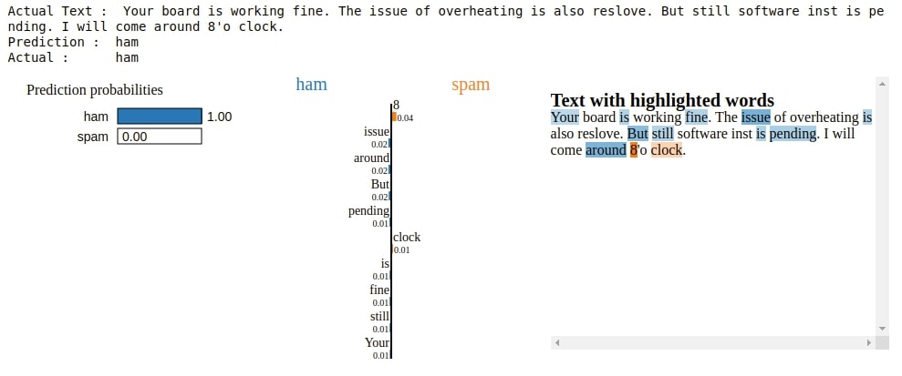
We have now taken a random test text example and created an explanation object for the same. We have passed function created earlier to classifier_fn parameter of explain_instance() method of LimeTextExplainer object.

There is another way to do the same thing if we don't want to create a function and want to use our default predict_proba() function of random forest. We can pass TF-IDF transformed (X_test_tfidf) random sample instead of actual text sample to explain_instance() method and reference rf.predict_proba to classifier_fn parameter and it'll generate the same results.

The visualization for text dataset shows actual text with words highlighted. We can see from explanation words that contribute positively to prediction and words that contribute negatively.

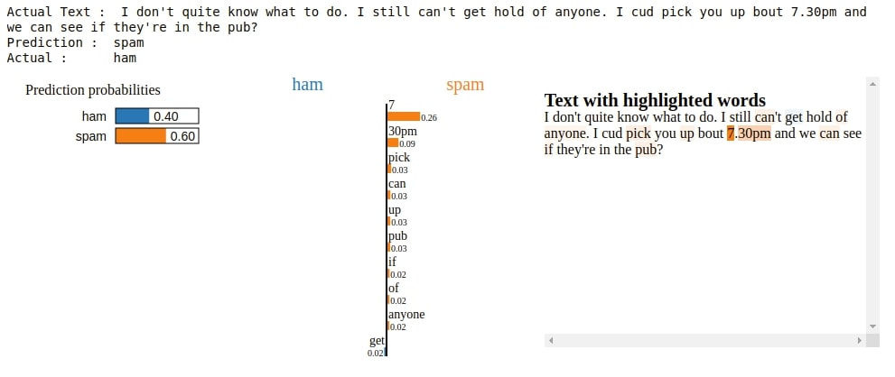
4. Explain Incorrect Predictions¶

Below we have explained another random text example from test data but this time we have chosen a random text example for which model makes the wrong prediction to understand which words are contributing to the wrong prediction. This can give us more confidence in model performance.

6. "lime_image": LIME For Unstructured Data ("Image") ¶

The third module that we'll be explaining for the lime library is 'lime_image' which provides an explainer that can help us generate an explanation for images. We'll be using the digits dataset to explain how to generate an explanation using this module.

6.1 Digits Multi-Class Image Classification¶

The example that we'll use for explaining the usage of the 'lime_image' module is a classification of digits dataset. The digits dataset is easily available from scikit-learn. It has images of size 8x8 for digits 0-9.

6.1.1 Load Dataset, Train Model and Calculate ML Metrics¶

Below, we have loaded digits dataset, divided it into train/test sets, fitted gradient boosting classifier to train data, and generated classification metrics like accuracy, confusion matrix, and classification report on the test dataset.

We can notice from the metrics results that our model is doing a good job. Next, we'll explain individual predictions using "lime".

6.1.2 Explain Individual Prediction using "LimeImageExplainer"¶

1. Create "LimeImageExplainer" Object¶

The LimeImageExplainer available as a part of the 'lime_image' module can help us explain images by highlighting which parts of the image have contributed to the prediction of a particular class.

Here are some of the important parameters of LimeImageExplainer.

• feature_selection - It accepts a string value from below list for feature selection when selecting the m-best feature as described in the internal working of LIME earlier.
  • 'forward_selection'
  • 'lasso_path'
  • 'none'
  • 'auto'
• random_state - It accepts integer or np.RandomState object specifying random state so that we can reproduce the same results each time we rerun the process.

Below we have created an instance of LimeImageExplainer which we'll use for explaining images classified using gradient boosting classifier and which part (pixels) of the image contributed to that prediction.

2. Define Prediction Function¶

Below we have created a function that takes a list of RGB images as input, transforms them into grayscale images, and then returns probabilities of that images using a gradient boosting classifier.

The reason for designing this method is that it'll be used when explaining the random image.

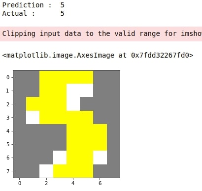
3. Explain Correct Predictions¶

Below we have taken a random image from the test dataset. Then, we have generated an explanation instance for that image by passing the image to the explain_instance() method of explainer object. We have also passed a reference to the prediction function which we designed earlier to the classifier_fn parameter.

If your images are RGB then you don't need to do any transformation.

We have then called get_image_and_mask() method on explanation object. This method takes as input actual label for which we want an explanation (highlight part of the image which contributed to predicting that label) and returns two arrays.

• actual_image -3D numpy array
• mask - 2D numpy array. It has pixels highlighted that contribute to prediction.

We can then combine this image and mask to check which pixels contributed to the prediction.

Below are some of the important parameters of get_image_and_mask() method.

• label - It accepts the class label that we want to explain.
• positive_only - It accepts boolean value specifying whether to take only superpixels that contributed positively to the prediction or not. The default is True.
• negative_only - It accepts boolean value specifying whether to take only superpixels that contributed negatively to the prediction or not. The default is False.
• hide_rest - It accepts boolean value specifying whether to return pixels that do not contribute to prediction or gray out them. The default is False.
• num_features - It accepts integers specifying the number of superpixels to include in explanation. The default is 5.

Below we have combined images generated by get_image_and_mask() to generate a single image highlighting which pixels contributed to prediction.

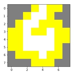
Below we have generated an explanation for another random test sample. We have tweaked a few parameters of method get_image_and_mask() for an explanation.

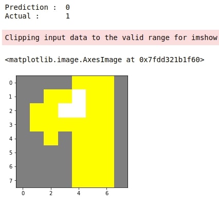
4. Explain Incorrect Predictions¶

Below we have generated an explanation for another random image from test data for which our model got the wrong prediction.

This ends our small tutorial explaining how we can use Python library 'lime' for interpreting predictions made by our ML Models. We explained various explainers available from 'lime' for interpreting model predictions for different kinds of data like structured data (tabular), text data, and image data.

References ¶

1. How to Use LIME for Deep Neural Networks?¶

1.1. Text Data¶

• LIME: Interpret Predictions of Flax(JAX) Text Classification Networks
• LIME: Interpret Predictions of Keras Text Classification Networks

1.2. Image Data¶

• LIME: Explain Keras Image Classification Network Predictions

2. LIME Implementation in Eli5 Library¶

• Eli5.lime: Explain PyTorch Text Classification Network Predictions
• Eli5.lime: Interpret Flax (JAX) Text Classifier Predictions using LIME

3. Other ML Model Interpretation Libraries¶

• How to Use eli5 to Understand sklearn Models, their Performance, and their Predictions?
• Treeinterpreter - Interpreting Tree-Based Model's Prediction of Individual Sample
• SHAP - Explain Machine Learning Model Predictions using Game Theoretic Approach
• interpret-text - Interpret NLP Models and Their Predictions
• dice-ml - Diverse Counterfactual Explanations for ML Models
• interpret-ml - Explain Machine Learning Models and Their Predictions

4. Other Libraries used in Tutorial¶

• Yellowbrick - Text Data Visualizations
• Yellowbrick - Visualize Sklearn's Classification & Regression Metrics in Python
• Scikit-Plot: Visualizing Machine Learning Algorithm Results and Performance
• Feature Extraction from Text Data using Scikit-Learn
• Model Evaluation Metrics in Scikit-Learn

5. Video Explaining How LIME Works¶

• Interpretable Machine Learning Using LIME Framework - Kasia Kulma (Ph.D.), Data Scientist, Aviva