LIME: Interpret Predictions Of Flax (JAX) Text Classification Networks
Nowadays, it's quite common to interpret the predictions made by neural networks and explain why networks made a certain prediction. It's very important to know which parts of data were used for decision-making for the generalization of our network. Let's say for image classification tasks, we want that the network is using pixels where actual objects are present to classify it to a particular category. The same goes for text classification tasks, where we want that network is using words that make sense to classify documents into a particular category. Many times, it might happen that our network is giving good accuracy but it's not catching actual patterns in data that it should catch to make decisions, and patterns that make sense should be used for decision making. There are various algorithms and libraries available that let us explain the predictions made by our models. We'll be concentrating on LIME (Local Interpretable Model-Agnostic Explanations) algorithm in this tutorial.
As a part of this tutorial, we'll explain how we can use LIME to explain the predictions made by our text classification network designed using Flax (JAX). We have used 20 newsgroups dataset available from scikit-learn for our purpose and vectorized that text data in different ways. Then, we have trained a simple network on vectorized data and explained predictions made by it. We assume that the reader has little background on LIME and text classification using neural networks. Please feel free to check the below links if you want to learn about them. We have covered how LIME algorithm works internally in detail over there.
- How to Use LIME to Understand Scikit-Learn Model's Predictions?
- Text Classification Using Flax (JAX) Networks
Below, we have listed important sections of tutorial to give an overview of the material covered.
Important Sections Of Tutorial
- Load Data
- Word Frequency Count Model
- Vectorize Text Data
- Define Flax (JAX) Classification Network
- Define Loss Function
- Train Network
- Evaluate Network Performance
- Explain Network Predictions
- Explain Correct Predictions
- Explain Incorrect Predictions
- Word Frequency Count Model (Stop Words Removed)
- Vectorize Text Data
- Train Network
- Explain Network Predictions
- Explain Correct Predictions
- Explain Incorrect Predictions
- TfIdf (Term Frequency-Inverse Document Frequency) Model
- TfIdf Model (Stop Words Removed)
Below, we have imported the necessary libraries and printed the versions that we have used in our tutorial.
import jax

print("JAX Version : {}".format(jax.__version__))
import flax

print("FLAX Version : {}".format(flax.__version__))
import optax

print("OPTAX Version : {}".format(optax.__version__))
Load Data 
In this section, we have loaded the 20 newsgroups dataset available from scikit-learn. The dataset has ~18k text documents for 20 different categories. As a part of our tutorial, we'll be using only 5 categories to keep things simple. We have listed below 5 categories that we'll use in code. Scikit-learn provides a method named fetch_20newsgroups() that let us load data. It let us load train and test sets differently.
Once data is loaded, we'll vectorize text data in different ways and train models on them. We'll then use lime to understand predictions made on the vectorized datasets.
import numpy as np
from sklearn import datasets
import gc

all_categories = ['alt.atheism','comp.graphics','comp.os.ms-windows.misc','comp.sys.ibm.pc.hardware',
                  'comp.sys.mac.hardware','comp.windows.x', 'misc.forsale','rec.autos','rec.motorcycles',
                  'rec.sport.baseball','rec.sport.hockey','sci.crypt','sci.electronics','sci.med',
                  'sci.space','soc.religion.christian','talk.politics.guns','talk.politics.mideast',
                  'talk.politics.misc','talk.religion.misc']

selected_categories = ['misc.forsale','rec.autos','rec.sport.baseball','sci.electronics','soc.religion.christian']

X_train_text, Y_train = datasets.fetch_20newsgroups(subset="train", categories=selected_categories, return_X_y=True)
X_test_text , Y_test  = datasets.fetch_20newsgroups(subset="test", categories=selected_categories, return_X_y=True)

X_train_text = np.array(X_train_text)
X_test_text = np.array(X_test_text)

classes = np.unique(Y_train)
mapping = dict(zip(classes, selected_categories))

len(X_train_text), len(X_test_text), classes, mapping
1. Word Frequency Count Model 
In this section, we are using an approach that keeps track of the frequency of the word in a document. We have used count vectorizer available from scikit-learn that lets converts of text documents to a list of floats where floats are frequencies of words.
Please make a NOTE that we have not covered how text vectorization works in detail as we have already covered them in the below link. Please feel free to check it if you want to know in detail how text vectorization works. It covers all approaches that we have used in our tutorial.
Vectorize Text Data
In this section, we have vectorized our train and text documents using CountVectorizer() available from scikit-learn. After vectorizing data, we have also converted it to JAX arrays as required by Flax/JAX networks.
import sklearn
from jax import numpy as jnp
from sklearn.feature_extraction.text import CountVectorizer

vectorizer = CountVectorizer(max_features=50000)

vectorizer.fit(np.concatenate((X_train_text, X_test_text)))
X_train = vectorizer.transform(X_train_text)
X_test = vectorizer.transform(X_test_text)

X_train = jnp.array(X_train.toarray(), dtype=jnp.float16)
X_test  = jnp.array(X_test.toarray(), dtype=jnp.float16)

X_train.shape, X_test.shape
import gc

gc.collect()
Define Flax (JAX) Classification Network
In this section, we have designed a network of the dense layers using Flax that we'll use to classify our text documents by training them on vectorized data. The network has 3 dense layers with 128, 64, and 5 (number of target classes) units respectively.
Please feel free to check the below link if you want to learn about Flax and how to create networks using it.
from flax import linen
from jax import random

class TextClassifier(linen.Module):
    def setup(self):
        self.linear1 = linen.Dense(features=128, name="DENSE1")
        self.linear2 = linen.Dense(features=64, name="DENSE2")
        self.linear3 = linen.Dense(len(classes), name="DENSE3")

    def __call__(self, inputs):
        x = linen.relu(self.linear1(inputs))
        x = linen.relu(self.linear2(x))
        logits = self.linear3(x)

        return logits #linen.softmax(x)
Define Loss Function
In this section, we have defined a function that we'll use as our loss function. We'll be using cross entropy loss for our case. The function takes network parameters, input data, and actual target values as input. It then takes network parameters and makes predictions on input data. It then one hot encodes actual target values and calculates cross-entropy loss using softmax_cross_entropy() function available from Optax library by giving one-hot encoded target and predictions.
def CrossEntropyLoss(weights, input_data, actual):
    logits_preds = model.apply(weights, input_data)
    one_hot_actual = jax.nn.one_hot(actual, num_classes=len(classes))
    return optax.softmax_cross_entropy(logits=logits_preds, labels=one_hot_actual).sum()
Train Network
In this section, we have trained our network so that we can use it later to make predictions. In order to train the network, we have designed a simple function. The function takes train data (X, Y), validation data (X_val, Y_val), number of epochs, network parameters, optimizer state, and batch size as input. It then executes the training loop number of epochs time. For each epoch, it loops through training data in batches calculating loss, calculating gradients, and updating weights. It prints training loss and validation accuracy at the end of each epoch. The function returns updated network parameters at last.
from jax import value_and_grad
from tqdm import tqdm
from sklearn.metrics import accuracy_score

def TrainModelInBatches(X, Y, X_val, Y_val, epochs, weights, optimizer_state, batch_size=32):
    for i in range(1, epochs+1):
        batches = jnp.arange((X.shape[0]//batch_size)+1) ### Batch Indices

        losses = [] ## Record loss of each batch
        for batch in tqdm(batches):
            if batch != batches[-1]:
                start, end = int(batch*batch_size), int(batch*batch_size+batch_size)
            else:
                start, end = int(batch*batch_size), None

            X_batch, Y_batch = X[start:end], Y[start:end] ## Single batch of data

            loss, gradients = value_and_grad(CrossEntropyLoss)(weights, X_batch,Y_batch)

            ## Update Weights
            updates, optimizer_state = optimizer.update(gradients, optimizer_state)
            weights = optax.apply_updates(weights, updates)

            losses.append(loss) ## Record Loss

        print("CrossEntropyLoss : {:.3f}".format(jnp.array(losses).mean()))

        Y_val_preds = model.apply(weights, X_val)
        val_acc = accuracy_score(Y_val, jnp.argmax(Y_val_preds, axis=1))
        print("Validation  Accuracy : {:.3f}".format(val_acc))

    return weights
Below, we have actually trained our network using the function designed in the previous cell. We have initialized batch size to 256, epochs to 8, and learning rate to 0.001. Then, we have initialized the classifier and its parameters. Followed by it, we have initialized Adam optimizer available from Optax library and optimizer state by giving network parameters. At last, we have called our training routine by giving the required parameters to train the network. We can notice from the loss and accuracy getting printed after each epoch that our model seems to be doing a good job.
seed = random.PRNGKey(0)
batch_size=256
epochs=8
learning_rate = jnp.array(1/1e3)

model = TextClassifier()
weights = model.init(seed, X_train[:5])

optimizer = optax.adam(learning_rate=learning_rate)
optimizer_state = optimizer.init(weights)

final_weights = TrainModelInBatches(X_train, Y_train, X_test, Y_test, epochs, weights, optimizer_state, batch_size=batch_size)
Evaluate Network Performance
In this section, we have evaluated the performance of our network by calculating accuracy, classification report and confusion matrix metrics. We have first made predictions using a trained network and then calculated metrics using actual and prediction values. We have used various functions available from scikit-learn to calculate these metrics.
Please feel free to check the below link if you want to learn about various ML metrics available from scikit-learn as it covers the majority of them in detail.
from sklearn.metrics import accuracy_score, classification_report, confusion_matrix

train_preds = model.apply(final_weights, X_train)
test_preds = model.apply(final_weights, X_test)

print("Train Accuracy : {:.3f}".format(accuracy_score(Y_train, np.argmax(train_preds, axis=1))))
print("Test  Accuracy : {:.3f}".format(accuracy_score(Y_test, np.argmax(test_preds, axis=1))))
print("\nClassification Report : ")
print(classification_report(Y_test, np.argmax(test_preds, axis=1), target_names=selected_categories))
print("\nConfusion Matrix : ")
print(confusion_matrix(Y_test, np.argmax(test_preds, axis=1)))
Explain Network Predictions
In this section, we have explained the predictions made by the network using lime. We have explained both correct predictions and incorrect predictions to analyze which words are contributing to the prediction.
In order to explain predictions using lime, we need to create an instance of LimeTextExplainer which we can use later to explain predictions by calling explain_instance() function on it. The explain_instance() function returns Explanation object which can be visualized by calling show_in_notebook() method on it.
We suggest that you go through our tutorial on lime below where we have explained various arguments taken by LimeTextExplainer() constructor.
from lime import lime_text

explainer = lime_text.LimeTextExplainer(class_names=selected_categories, verbose=True)

explainer
Explain Correct Predictions
In this section, we have explained correct prediction made by our model by calling explain_instance() function on LimeTextExplainer object.
Below, we have first created a simple function that takes as input text samples and returns class probabilities of those samples. It first vectorizes data using a vectorizer and then performs a forward pass through the network to make predictions. The predictions are converted to probabilities and returned from the function.
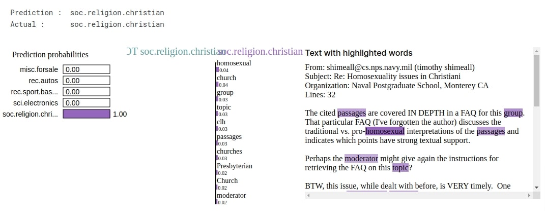
After defining a function, we have taken a random sample from test data and made predictions on it. We have also printed the actual and predicted label of the sample. The actual label of the sample was 'soc.religion.christian' and our model predicted the same.
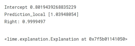
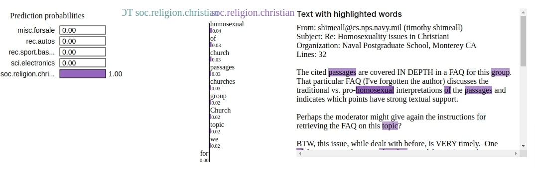
Then, in the next cell, we have called explain_instance() method on LimeTextExplainer object. We have given a text sample, a function that returns probabilities, and an actual label to a method. It returns Explanation object on which we have called show_in_notebook() method in the next cell to display a visualization that explains predictions. The visualizations show a bar chart showing which words contributed to predictions. It also shows the actual sample highlighted with words that contributed to prediction.
We can notice from the visualization that words like 'homosexual', 'church', 'group', etc are contributing to predicting label 'soc.religion.christian'.
import numpy as np

def make_predictions(X_batch_text):
    X_batch = vectorizer.transform(X_batch_text)
    logits = model.apply(final_weights, jnp.array(X_batch.toarray()))
    preds = linen.softmax(logits)
    return preds.to_py()

rng = np.random.RandomState(42)
idx = rng.randint(1, len(X_test))

print("Prediction : ", selected_categories[model.apply(final_weights, X_test[idx:idx+1]).argmax(axis=-1)[0]])
print("Actual :     ", selected_categories[Y_test[idx]])
explanation = explainer.explain_instance(X_test_text[idx], classifier_fn=make_predictions,
                                         labels=Y_test[idx:idx+1])

explanation
explanation.show_in_notebook()
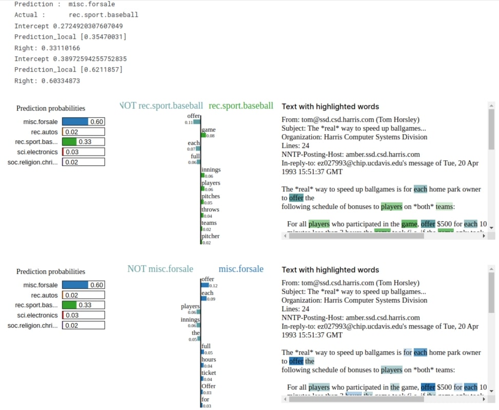
Explain Incorrect Predictions
In this section, we have explained incorrect predictions made by our model.
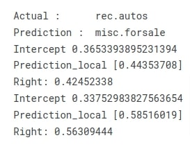
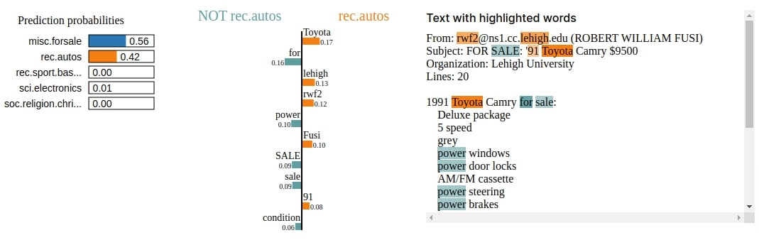
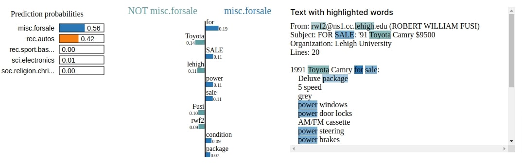
We have first found out indexes of wrong predictions from test data. Then, we have selected one sample from test data for which our model predicts the wrong target label. The actual label of the selected sample is 'rec.autos' and our model predicts 'misc.forsale'.
Then, we have created two explanation objects for that wrong prediction (one with respect to the actual label and one with respect to the predicted label) using explain_instance() function. This will help us understand which words contributed to both categories. We have visualized both explanations in the next cells.
We can notice from first visualization that words like 'Toyota', 'Lehigh', etc are contributing to category 'rec.autos' and words like 'sale', 'condition', 'package', 'power', etc are contributing to category 'misc.forsale'. We can also notice that there is not much difference in the probability of both categories as the model is not much sure about any of them.
import numpy as np

Y_test_preds = np.argmax(test_preds, axis=-1)
wrong_preds = np.argwhere(Y_test!=Y_test_preds)

rng = np.random.RandomState(123)
idx = rng.choice(wrong_preds.flatten())

print("Actual :     ", selected_categories[Y_test[idx]])
print("Prediction : ", selected_categories[model.apply(final_weights, X_test[idx:idx+1]).argmax(axis=-1)[0]])

explanation_actual = explainer.explain_instance(X_test_text[idx], classifier_fn=make_predictions,
                                                labels=Y_test[idx:idx+1])
explanation_pred = explainer.explain_instance(X_test_text[idx], classifier_fn=make_predictions,
                                              labels=Y_test_preds[idx:idx+1].to_py())
explanation_actual.show_in_notebook()
explanation_pred.show_in_notebook()
2. Word Frequency Count (Stop Words Removed) 
In this section, we have again used the word frequency count approach but this time we have used commonly appearing words in the English language like 'the', 'a' ,'an', etc when vectorizing text data. The majority of the code in this section is the same as the previous section. Only, the approach to vectorize data is different. This will help us better understand whether this approach gives good results.
Vectorize Text Data
In this section, we have vectorized our data again using scikit-learn's CountVectorizer. The code is exactly the same as our earlier vectorization from the previous section with the only difference that we have asked the vectorizer to remove commonly appearing stop words by providing stop_words parameter with value 'english'.
import sklearn
import numpy as np
from sklearn.feature_extraction.text import CountVectorizer

vectorizer = CountVectorizer(max_features=50000, stop_words="english")

vectorizer.fit(np.concatenate((X_train_text, X_test_text)))
X_train = vectorizer.transform(X_train_text)
X_test = vectorizer.transform(X_test_text)

X_train = jnp.array(X_train.toarray(), dtype=jnp.float16)
X_test  = jnp.array(X_test.toarray(), dtype=jnp.float16)

X_train.shape, X_test.shape
Train Network
In this section, we have trained our network with data vectorized in the previous cell. All the settings are exactly the same as the previous section with only changes in input data which is vectorized using a different approach as explained earlier. We can notice from the training loss and validation accuracy getting printed after each epoch that results are almost the same as the previous section.
seed = random.PRNGKey(0)
batch_size=256
epochs=8
learning_rate = jnp.array(1/1e3)

model = TextClassifier()
weights = model.init(seed, X_train[:5])

optimizer = optax.adam(learning_rate=learning_rate)
optimizer_state = optimizer.init(weights)

final_weights = TrainModelInBatches(X_train, Y_train, X_test, Y_test, epochs, weights, optimizer_state, batch_size=batch_size)
Explain Network Predictions
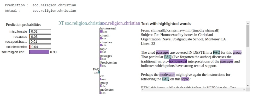
Explain Correct Predictions
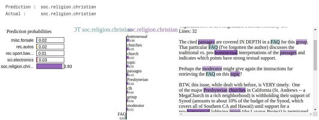
In this section, we have explained one correct prediction. The actual label of our selected sample is 'soc.religion.christian' and the predicted label is the same. We can notice from the visualization that words like 'homosexual', 'church', 'group', 'passages', 'presbyterian', 'moderator', etc are contributing to predicting the label. We can notice that results are a little better compared to our previous approach as it is detecting more words that can exactly define a category.
The majority of the code in this section is just a repeat of our previous section.
import numpy as np

def make_predictions(X_batch_text):
    X_batch = vectorizer.transform(X_batch_text)
    logits = model.apply(final_weights, jnp.array(X_batch.toarray()))
    preds = linen.softmax(logits)
    return preds.to_py()

rng = np.random.RandomState(42)
idx = rng.randint(1, len(X_test))

print("Prediction : ", selected_categories[model.apply(final_weights, X_test[idx:idx+1]).argmax(axis=-1)[0]])
print("Actual :     ", selected_categories[Y_test[idx]])

explainer = lime_text.LimeTextExplainer(class_names=selected_categories)

explanation = explainer.explain_instance(X_test_text[idx], classifier_fn=make_predictions, labels=Y_test[idx:idx+1])

explanation.show_in_notebook()
Explain Incorrect Predictions
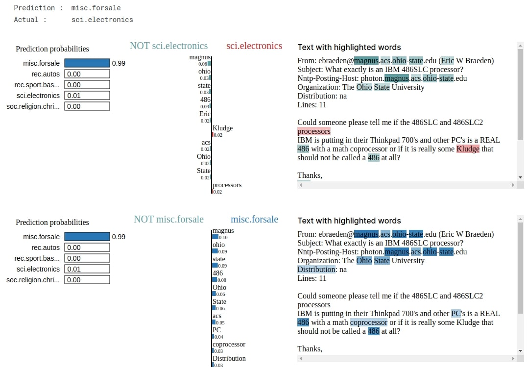
In this section, we have explained one wrong prediction. The actual label of the selected sample is 'sci.electronics' and the label predicted by our model is 'misc.forsale'.
Y_test_preds = model.apply(final_weights, X_test).argmax(axis=-1)
wrong_preds = np.argwhere(Y_test!=Y_test_preds)
rng = np.random.RandomState(42)
idx = rng.choice(wrong_preds.flatten())

print("Prediction : ", selected_categories[model.apply(final_weights, X_test[idx:idx+1]).argmax(axis=-1)[0]])
print("Actual :     ", selected_categories[Y_test[idx]])

explainer = lime_text.LimeTextExplainer(class_names=selected_categories)

explanation_actual = explainer.explain_instance(X_test_text[idx], classifier_fn=make_predictions,
                                                num_features=10, labels=Y_test[idx:idx+1])
explanation_pred = explainer.explain_instance(X_test_text[idx], classifier_fn=make_predictions,
                                              num_features=10, labels=Y_test_preds[idx:idx+1].to_py())

explanation_actual.show_in_notebook()
explanation_pred.show_in_notebook()
3. TfIdf (Term Frequency-Inverse Document Frequency) Model 
In this section, we have used another approach called Tf-IDF (Term Frequency - Inverse Document Frequency) to vectorize our text data. The approach generates float values per word of the document in a way that words that commonly appear are given less importance and words that appear rarely per text document are given more importance to improve results.
Please feel free to check our tutorial on feature extraction from text data that covers the approach in detail.
Vectorize Text Data
In this section, we have vectorized our data using TfidfVectorizer available from scikit-learn. The majority of the code is the same as the previous section with only a difference in the vectorizer.
import sklearn
import numpy as np
from sklearn.feature_extraction.text import TfidfVectorizer

vectorizer = TfidfVectorizer(max_features=50000)

vectorizer.fit(np.concatenate((X_train_text, X_test_text)))
X_train = vectorizer.transform(X_train_text)
X_test = vectorizer.transform(X_test_text)

X_train = jnp.array(X_train.toarray(), dtype=jnp.float16)
X_test  = jnp.array(X_test.toarray(), dtype=jnp.float16)

X_train.shape, X_test.shape
Train Network
Below, we have trained our network using the data vectorized using Tf-Idf approach. All the settings are the same as our previous section with only a change in data which is vectorized using a different approach. We can notice from the training loss and validation accuracy getting printed after each epoch that this model has done a better job compared to our previous models.
seed = random.PRNGKey(0)
batch_size=256
epochs=8
learning_rate = jnp.array(1/1e3)

model = TextClassifier()
weights = model.init(seed, X_train[:5])

optimizer = optax.adam(learning_rate=learning_rate)
optimizer_state = optimizer.init(weights)

final_weights = TrainModelInBatches(X_train, Y_train, X_test, Y_test, epochs, weights, optimizer_state, batch_size=batch_size)
Explain Network Predictions
Explain Correct Predictions
In this section, we have explained one correct prediction as usual. The actual category of sample is 'soc.religion.christian' and our model also predicts the same. It is detecting almost the same words as our previous model to identify category 'soc.religion.christian'.
import numpy as np

def make_predictions(X_batch_text):
    X_batch = vectorizer.transform(X_batch_text)
    logits = model.apply(final_weights, jnp.array(X_batch.toarray()))
    preds = linen.softmax(logits)
    return preds.to_py()

rng = np.random.RandomState(42)
idx = rng.randint(1, len(X_test))

print("Prediction : ", selected_categories[model.apply(final_weights, X_test[idx:idx+1]).argmax(axis=-1)[0]])
print("Actual :     ", selected_categories[Y_test[idx]])

explainer = lime_text.LimeTextExplainer(class_names=selected_categories)

explanation = explainer.explain_instance(X_test_text[idx], classifier_fn=make_predictions,
                                         labels=Y_test[idx:idx+1])

explanation.show_in_notebook()
Explain Incorrect Predictions
In this section, we have explained one wrong prediction. The actual category of our selected sample is 'rec.sport.baseball' and our model predicted 'misc.forsale'.
Y_test_preds = model.apply(final_weights, X_test).argmax(axis=-1)
wrong_preds = np.argwhere(Y_test!=Y_test_preds)
rng = np.random.RandomState(42)
idx = rng.choice(wrong_preds.flatten())

print("Prediction : ", selected_categories[model.apply(final_weights, X_test[idx:idx+1]).argmax(axis=-1)[0]])
print("Actual :     ", selected_categories[Y_test[idx]])

explainer = lime_text.LimeTextExplainer(class_names=selected_categories, verbose=True)

explanation_actual = explainer.explain_instance(X_test_text[idx], classifier_fn=make_predictions,
                                                num_features=10, labels=Y_test[idx:idx+1])
explanation_pred = explainer.explain_instance(X_test_text[idx], classifier_fn=make_predictions,
                                              num_features=10, labels=Y_test_preds[idx:idx+1].to_py())

explanation_actual.show_in_notebook()
explanation_pred.show_in_notebook()
4. TfIdf Model (Stop Words Removed) 
In this section, we have again used Tf-Idf approach but we have removed stop words from our data. The majority of the code in this section is just a repeat of previous examples with only minor changes in text vectorization.
Vectorize Text Data
Below, we have again vectorized text data using TfidfVectorizer but this time we have asked it to remove stop words by setting stop_words argument's value to 'english'. The rest of the code is almost the same as our previous examples.
import sklearn
import numpy as np
from sklearn.feature_extraction.text import TfidfVectorizer

vectorizer = TfidfVectorizer(max_features=50000, stop_words="english")

vectorizer.fit(np.concatenate((X_train_text, X_test_text)))
X_train = vectorizer.transform(X_train_text)
X_test = vectorizer.transform(X_test_text)

X_train = jnp.array(X_train.toarray(), dtype=jnp.float16)
X_test  = jnp.array(X_test.toarray(), dtype=jnp.float16)

X_train.shape, X_test.shape
Train Network
In this section, we have trained our network using data vectorized in the previous cell. As per loss and validation accuracy, results are a little low compared to our previous text vectorization approaches.
seed = random.PRNGKey(0)
batch_size=256
epochs=8
learning_rate = jnp.array(1/1e3)

model = TextClassifier()
weights = model.init(seed, X_train[:5])

optimizer = optax.adam(learning_rate=learning_rate)
optimizer_state = optimizer.init(weights)

final_weights = TrainModelInBatches(X_train, Y_train, X_test, Y_test, epochs, weights, optimizer_state, batch_size=batch_size)
Explain Network Predictions
Explain Correct Predictions
In this section, we have explained one correct prediction whose label is 'soc.religion.christian'. We can notice from the visualization that as usual words like 'homosexual', 'church', 'passages', 'presbyterian', etc are contributing to label 'soc.religion.christian'.
import numpy as np

def make_predictions(X_batch_text):
    X_batch = vectorizer.transform(X_batch_text)
    logits = model.apply(final_weights, jnp.array(X_batch.toarray()))
    preds = linen.softmax(logits)
    return preds.to_py()

rng = np.random.RandomState(42)
idx = rng.randint(1, len(X_test))

print("Prediction : ", selected_categories[model.apply(final_weights, X_test[idx:idx+1]).argmax(axis=-1)[0]])
print("Actual :     ", selected_categories[Y_test[idx]])

explainer = lime_text.LimeTextExplainer(class_names=selected_categories)

explanation = explainer.explain_instance(X_test_text[idx], classifier_fn=make_predictions,
                                         labels=Y_test[idx:idx+1])

explanation.show_in_notebook()
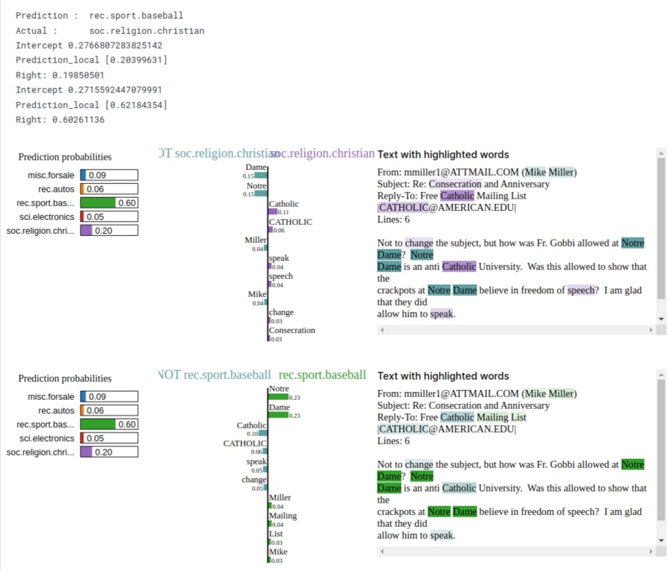
Explain Incorrect Predictions
In this section, we have explained one wrong prediction whose actual category is 'soc.religion.christian' and our model predicted 'rec.sport.baseball' which does not make sense. We can notice from the visualization that words contributed to making prediction 'rec.sport.baseball' does not make much sense and should not be part of that category. This signals us that we need to look at our model and need to improve it further for better performance.
Y_test_preds = model.apply(final_weights, X_test).argmax(axis=-1)
wrong_preds = np.argwhere(Y_test!=Y_test_preds)
rng = np.random.RandomState(42)
idx = rng.choice(wrong_preds.flatten())

print("Prediction : ", selected_categories[model.apply(final_weights, X_test[idx:idx+1]).argmax(axis=-1)[0]])
print("Actual :     ", selected_categories[Y_test[idx]])

explainer = lime_text.LimeTextExplainer(class_names=selected_categories, verbose=True)

explanation_actual = explainer.explain_instance(X_test_text[idx], classifier_fn=make_predictions,
                                                num_features=10, labels=Y_test[idx:idx+1])
explanation_pred = explainer.explain_instance(X_test_text[idx], classifier_fn=make_predictions,
                                              num_features=10, labels=Y_test_preds[idx:idx+1].to_py())

explanation_actual.show_in_notebook()
explanation_pred.show_in_notebook()
This ends our small tutorial explaining how we can use lime to explain predictions made by our Flax (JAX) text classification networks. Please feel free to let us know your views in the comments section.
References
 Sunny Solanki
Sunny Solanki
Intro: Software Developer | Youtuber | Bonsai Enthusiast
About: Sunny Solanki holds a bachelor's degree in Information Technology (2006-2010) from L.D. College of Engineering. Post completion of his graduation, he has 8.5+ years of experience (2011-2019) in the IT Industry (TCS). His IT experience involves working on Python & Java Projects with US/Canada banking clients. Since 2020, he’s primarily concentrating on growing CoderzColumn.
His main areas of interest are AI, Machine Learning, Data Visualization, and Concurrent Programming. He has good hands-on with Python and its ecosystem libraries.
Apart from his tech life, he prefers reading biographies and autobiographies. And yes, he spends his leisure time taking care of his plants and a few pre-Bonsai trees.
Contact: sunny.2309@yahoo.in


![YouTube Subscribe]() Comfortable Learning through Video Tutorials?
Comfortable Learning through Video Tutorials?
If you are more comfortable learning through video tutorials then we would recommend that you subscribe to our YouTube channel.
![Need Help]() Stuck Somewhere? Need Help with Coding? Have Doubts About the Topic/Code?
Stuck Somewhere? Need Help with Coding? Have Doubts About the Topic/Code?
 Stuck Somewhere? Need Help with Coding? Have Doubts About the Topic/Code?
When going through coding examples, it's quite common to have doubts and errors.
If you have doubts about some code examples or are stuck somewhere when trying our code, send us an email at coderzcolumn07@gmail.com. We'll help you or point you in the direction where you can find a solution to your problem.
You can even send us a mail if you are trying something new and need guidance regarding coding. We'll try to respond as soon as possible.
![Share Views]() Want to Share Your Views? Have Any Suggestions?
Want to Share Your Views? Have Any Suggestions?
 Want to Share Your Views? Have Any Suggestions?
If you want to
- provide some suggestions on topic
- share your views
- include some details in tutorial
- suggest some new topics on which we should create tutorials/blogs
 lime, text-classification, flax, jax