LIME: Interpret Predictions Of Keras Text Classification Networks¶

Interpreting the predictions of our ML model helps us better understand whether our model has generalized or not. It further opens up opportunities to understand what tasks model is doing good and at what tasks it's getting confused. This can help us make informed changes that can further improve model performance. We can easily generate feature importance for simple ML models like linear regression, decision trees, random forests, etc. But when it comes to deep neural networks, it becomes hard to generate feature importances specifying which features are contributing to the prediction. LIME (Local Interpretable Model-Agnostic Explanations) is an algorithm that helps us solve this problem. It can help us understand the prediction of our deep network by training simple ML models (like decision trees, linear regression, etc) on fake data generated from the input sample. This model tries to mimic the predictions of our network. We have covered in detail how LIME works internally in a separate tutorial. Please feel free to check the below link which has steps of internal workings.

• How to Use LIME to Understand sklearn Models Predictions?

As a part of this tutorial, we have used LIME to explain the predictions made by our text classification keras neural network. We have used the newsgroups text dataset available from scikit-learn for our purpose. The tutorial trains model on data vectorized with different text vectorization approach to see which one is doing a better job. We recommend that the reader goes through the below link if he/she does not have a background on text classification using keras networks.

• Text Classification Using Keras Networks

Below, we have listed important sections of tutorial to give an overview of the material covered.

Important Sections Of Tutorial¶

1. Network Using Keras Text Vectorization (Word Frequency)
   • Load Data
   • Vectorize Text Data
   • Create And Train Network
   • Evaluate Network Performance
   • Explain Network Predictions Using Lime
     • Explain Correct Predictions
     • Explain Incorrect Predictions
2. Network Using Scikit-Learn Text Vectorizer (Word Frequency)
   • Vectorize Text Data
   • Create And Train Model
   • Explain Network Predictions
     • Explain Correct Predictions
     • Explain Incorrect Predictions
3. Network Using Scikit-Learn Text Vectorizer (Word Frequency + Stop Words Removed)
4. Network Using Scikit-learn Text Vectorizer (Tf-Idf + Stop Words Removed)

Below, we have imported the necessary libraries and printed the versions that we have used in our tutorial.

1. Network Using Keras Text Vectorization (Word Frequency) ¶

In this section, we have vectorized our input text data using the word frequency approach and then trained a network on it. After training the network, we have evaluated its performance by calculating various ML metrics and explained predictions made by the network. We have used the text vectorization layer available from keras to vectorize data.

Load Data¶

In this section, we have loaded 20 newsgroups dataset that we'll be using throughout our tutorial. The dataset is available from scikit-learn and has ~18k text documents of 20 different categories. As a part of our example, we have selected 5 categories as listed in the code below. We have loaded train and test datasets using fetch_20newsgroups() function available from scikit-learn.

Vectorize Text Data¶

In this section, we have trained our text vectorization layer available from keras using our dataset. The training will populate the vocabulary of the vectorization layer. We'll later use this layer as a part of our keras network.

Create And Train Network¶

In this section, we have created a keras network which we'll use to classify text documents. The network consists of a text vectorization layer which we trained in the previous section to populate its dictionary followed by 3 dense layers. The three dense layers had 128, 64 AND 5 units respectively. The first two dense layers have relu activation and the last dense layer has softmax activation. When we perform a forward pass through the network, the first text vectorization layer will vectorize text data and pass vectorized data to the dense layer next. After creating a network, we have also summarized the network to show network parameters.

Then, we have compiled a network to use Adam optimizer, cross entropy loss, and accuracy metrics.

At last, we have called fit() method on the model to train it with train data for 8 epochs with a batch size of 256. We have also provided validation data to check the accuracy of the model on it.

Evaluate Network Performance¶

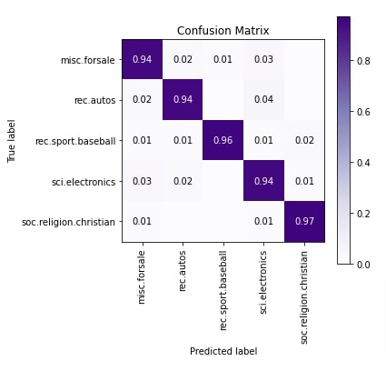
In this section, we have evaluated the performance of the network by calculating accuracy, classification report and confusion matrix metrics on the test dataset. We can notice from the results that our model seems to be doing a good job as per the accuracy metric. The model is confusing some samples of categories misc.forsale, rec.autos and sci.electronics as per confusion matrix.

We have calculated various ML metrics using functions available from scikit-learn. Please feel free to check the below link if you want to learn about them and others available through scikit-learn. It covers them in detail.

• Scikit-Learn - Model Evaluation & Scoring Metrics

In the next cell after the below cell, we have also plotted classification metrics using the scikit-plot python library. It provides visualizations for many ML metrics. Please feel free to check the below link if you want to learn about it.

• Scikit-Plot: Visualizing Machine Learning Algorithm Results And Performance

Explain Network Predictions Using Lime¶

In this section, we have explained the predictions made by our model using LIME algorithm. The lime library provides us with LimeTextExplainer that lets us explain predictions made by our model by creating visualizations that highlight words that contribute to the prediction category.

In order to explain predictions using lime, we first need to create an instance of LimeTextExplainer. Then, we need to call explain_instance() method on it with a sample to explain. The method returns an instance of Explanation on which we can call show_in_notebook() method to create visualization explaining prediction.

Below, we have first created an instance of LimeTextExplainer that we'll use to explain predictions. We have given it labels of all the output categories of our model.

We recommend that readers go through another simple tutorial on lime where we have covered arguments of LimeTextExplainer() constructor.

• LimeTextExplainer

Explain Correct Predictions¶

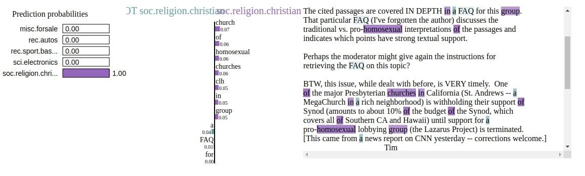
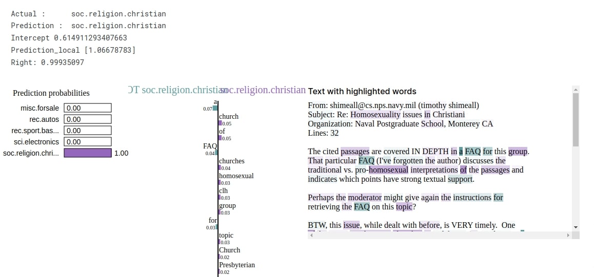
In this section, we have explained the correct prediction made by our model. We have first randomly selected one sample from the test data set. The category of the selected sample is soc.religion.christian and the same is predicted by our model.

Then, we have called explain_instance() function on LimeTabularExplainer instance by giving text sample, reference to predict() function of model and actual label of the sample. This returned an instance of Explanation which has sample explanation details.

At last, we have called show_in_notebook() function on explanation instance to show sample explanation. The visualization has a bar chart that shows which words contributed positively to the prediction categories as well as has original text of the sample with words highlighted showing whether they contributed positively or negatively to the prediction label. The words are highlighted as shades of color which are based on their contribution to prediction. We can notice from the visualization that words like 'church', 'homosexual', 'churches', 'group', etc are contributing to predicting category soc.religion.christian.

Explain Incorrect Predictions¶

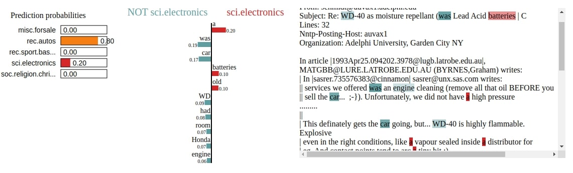
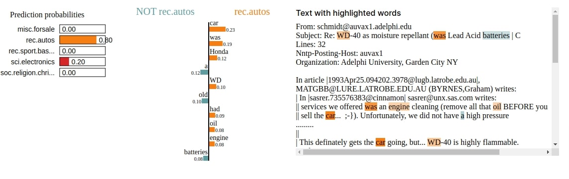
In this section, we have explained a wrong prediction using our explainer object. We have first found out indexes of all test samples that are predicted wrong by our model and then we have randomly selected one sample from it. The actual category of selected sample is sci.electronics and model predicted rec.autos. This time, we have generated two explanation objects (one with respect to the actual label and one with respect to the predicted label). This is done so that we can see which words are contributing to a particular category.

We can notice from the visualizations that words like 'batteries', 'old', etc contributed to predicting category sci.electronics and words like 'car', 'oil', 'engine', 'Honda', etc contributed to predicting category rec.autos.

Explain Correct Predictions¶

In this section, we have again explained the correct prediction but this time we have kept feature_selection parameter of LimeTextExplainer to 'none'.

2. Network Using Scikit-Learn Text Vectorizer (Word Frequency) ¶

In this section, we have again used the word frequency text vectorization approach but this time we have vectorized text data using CountVectorizer available from scikit-learn. Our keras network will be working directly on vectorized data this time.

Please NOTE that we have not covered text vectorization approaches that we have used in this tutorial in detail as we expect that reader has little background on them. Please feel free to check the below link if you want to learn about them in detail. The link covers them in detail.

• Scikit-Learn - Feature Extraction from Text Data

Vectorize Text Data¶

Below, we have vectorized our text data using CountVectorizer available from scikit-learn.

Create And Train Model¶

In this section, we have first created a keras network that works on vectorized data. It has 3 dense layers with units 128, 64, and 5 respectively.

After creating a network, we have compiled it to use Adam optimizer, cross entropy loss, and accuracy metrics.

At last, we have trained the network by calling fit() function for 8 epochs with a batch size of 256. We can notice from the loss and accuracy getting printed after each epoch that the model is doing a good job.

Explain Network Predictions¶

Explain Correct Predictions¶

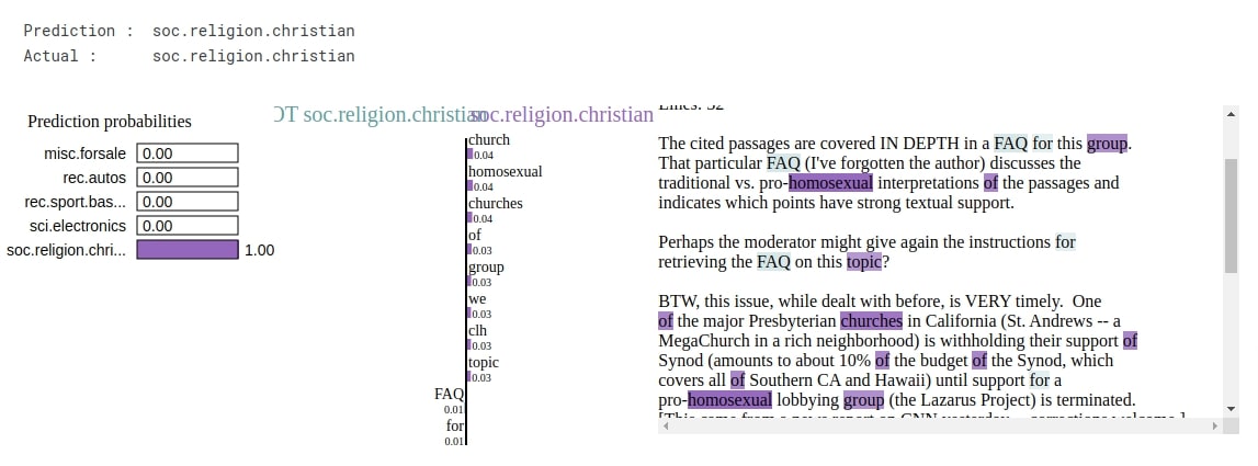
In this section, we have explained the correct prediction made by our model. We have randomly selected one sample from the test set. The actual and predicted category of that sample is soc.religion.christian.

This time we have created a small function that takes as input text samples and returns probabilities of those samples. This is required by classifier_fn parameter of explain_instance() function. In our previous example, we did not need to create such a function because our model was taking text samples as input and making predictions but in this example, it works on vectorized data hence we need to do it.

We can notice from the visualization that the words like 'church', 'homosexual', 'group', 'topic', etc are contributing to predicting category soc.religion.christian.

Explain Incorrect Predictions¶

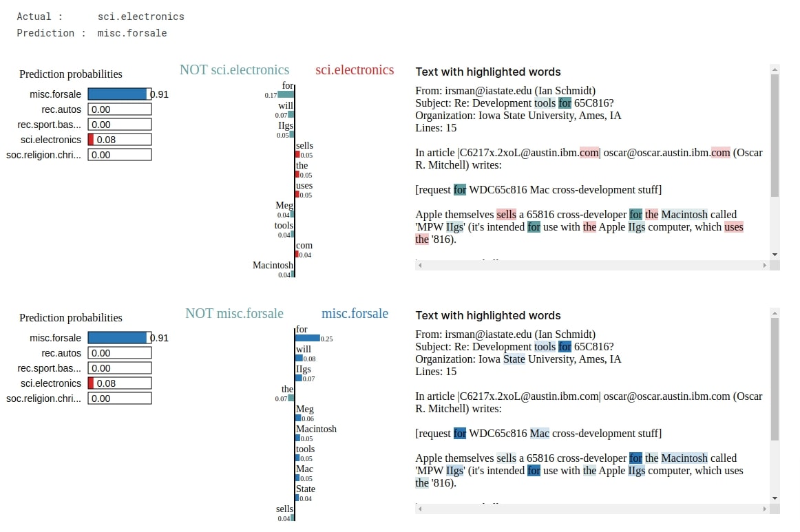
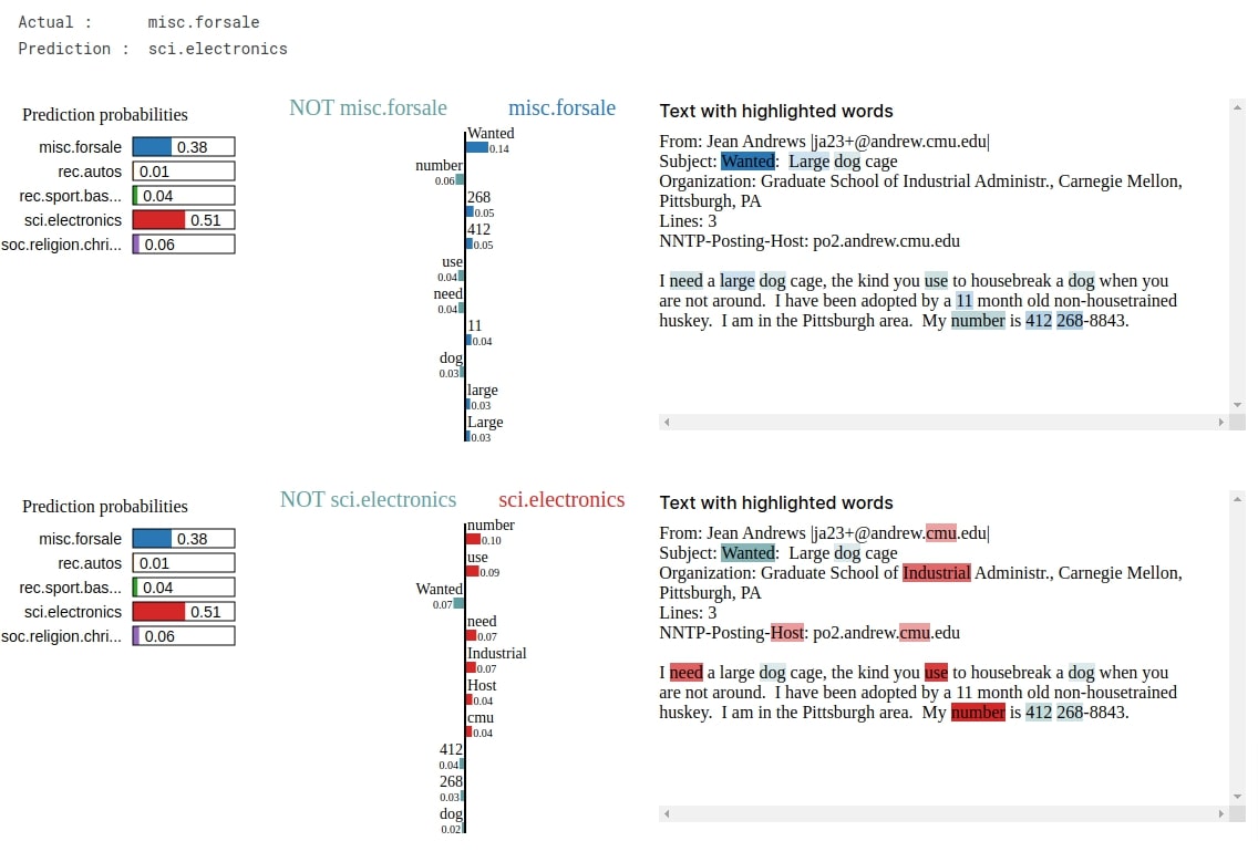
In this section, we have explained one wrong prediction. The actual category of our selected sample is sci.electronics whereas our model predicted misc.forsale. As usual, we have created two visualizations to see which words are contributing to actual and predicted labels.

We can notice that words like 'sells', 'com', etc are contributing to category sci.electronics whereas words like 'tools', 'Mac', 'Macintosh', etc are contributing to category misc.forsale. This does not make much sense as words that should be part of sci.electronics category are contributing to misc.forsale category. This hints that our model is not that generic enough.

3. Network Using Scikit-Learn Text Vectorizer (Word Frequency + Stop Words Removed) ¶

In this example, we have again used the word frequency approach but this time, we have removed commonly appearing words in the English language (words like 'the', 'a', 'an', 'then', etc) that do not contribute much to classification as they appear in almost every other text document. The majority of the code in this section is repeated from the previous section hence we have not included a detailed explanation of repeated parts.

Vectorize Text Data¶

In this section, we have vectorized data using scikit-learn CountVectorizer. We have set stop_words parameter to 'english' asking it to remove stop words from the vocabulary.

Create And Train Model¶

Here, we have created a model, compiled it, and trained it using vectorized data. We can notice from the loss and accuracy getting printed at the end of all epochs that the model is performing well.

Explain Network Predictions¶

Explain Correct Predictions¶

In this section, we have explained the correct prediction made by our model. The actual category of the selected sample is soc.religion.christian and the same is predicted by our model. The words like 'church', 'group', 'homosexual', 'presbyterian', etc are contributing to the prediction.

Explain Incorrect Predictions¶

In this section, we have explained one incorrect prediction. The actual category of the sample is 'misc.forsale' whereas our model predicted 'sci.electronics'. We have generated an explanation with respect to both actual and predicted labels.

4. Network Using Scikit-learn Text Vectorizer (Tf-Idf + Stop Words Removed) ¶

In this section, we have vectorized our data using Tf-Idf (Term Frequency-Inverse Document Frequency). It assigns float values to each word in a way that words that appear commonly across many documents get assigned low values and those appearing rarely get assigned high values.

Please feel free to check the below link if you want to learn about Tf-IDF in detail.

• Scikit-Learn - Feature Extraction from Text Data

Vectorize Text Data¶

In this section, we have vectorized data using TfidfVectorizer available from scikit-learn. The TfidfVectorizer is an implementation of Tf-IDF concept.

Create And Train Model¶

In this section, we have created and trained our model as usual. We can notice from the loss and accuracy that the model has done a good job at prediction.

Explain Network Predictions¶

Explain Correct Predictions¶

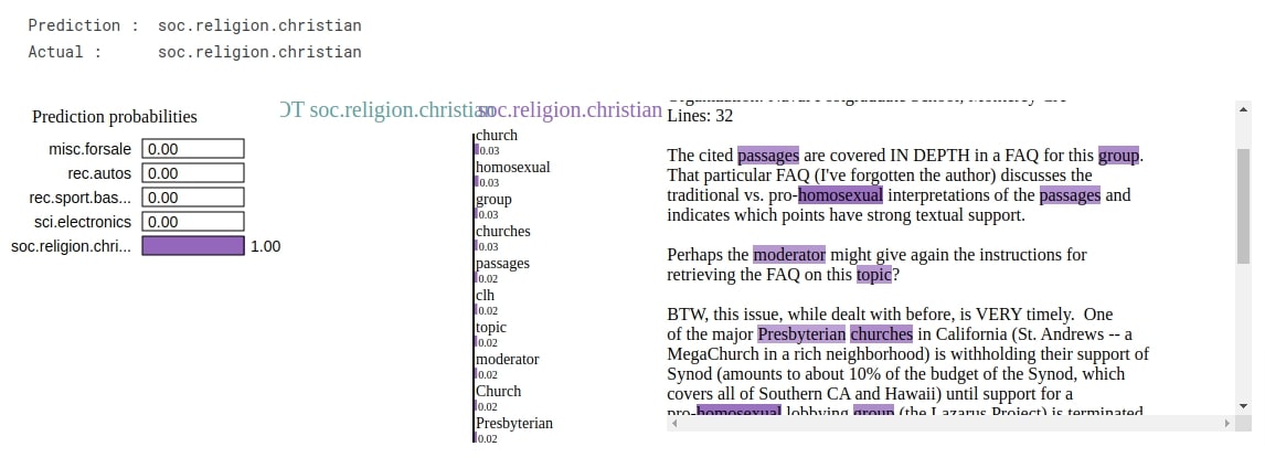
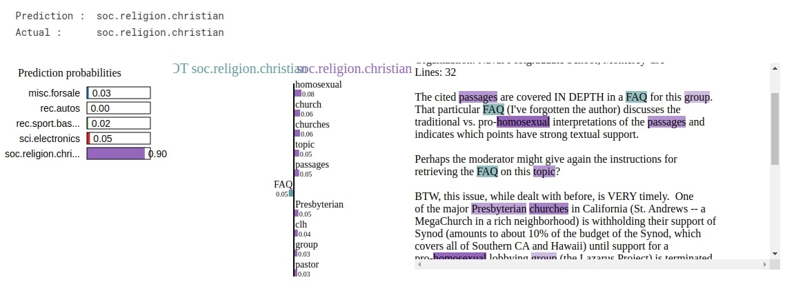
In this section, we have explained correct prediction. The model has predicted correct category soc.religion.christian. The words like 'homosexual', 'church', 'passages', 'group', 'presbyterian', etc contributed to prediction.

Explain Incorrect Predictions¶

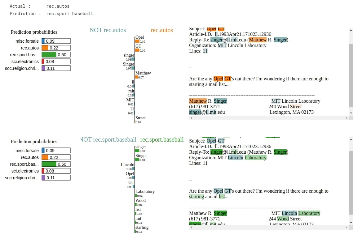
In this section, we have explained one incorrect prediction. The actual category of the selected sample is rec.autos whereas our model predicted rec.sport.baseball. We can check from visualizations which words contributed to a particular category.

This ends our small tutorial explaining how we can use lime to explain predictions made by our Keras text classification networks. Please feel free to let us know your views in the comments section.

References¶

• How to Use LIME to Understand sklearn Models Predictions?
• Text Classification Using Keras Networks
• Scikit-Learn - Feature Extraction from Text Data