treeinterpreter - Interpreting Tree-Based Model's Prediction of Individual Sample
Interpreting the prediction of the machine learning model has become very important nowadays to check the reliability of the model. The common machine learning metrics like accuracy, r2 score, mean squared error, roc AUC curve, precision-recall curve, etc and plotting of global weights of the model do not give us 100% confidence about the performance of the model. We might need to look into further which features contributed by how much in particular prediction. The global weights might not be useful in this situation when we need to answer about the contribution of an individual feature on a particular prediction. Finding out how a particular prediction contributed to a particular prediction can help us make a better decision, as well as help, check the reliability of model performance.
The treeinterpreter is one such library which can help us finding out contribution of individual feature on particular prediction for tree based models of scikit-learn. We'll be primarily focus on it by going through various examples. Currently, Treeinterpreter supports below mentioned scikit-learn models:
- DecisionTreeRegressor
- DecisionTreeClassifier
- ExtraTreeRegressor
- ExtraTreeClassifier
- RandomForestRegressor
- RandomForestClassifier
- ExtraTreesRegressor
- ExtraTreesClassifier
The treeinterpreter is based on a concept that when making a particular prediction decision tree or random forest follows a particular path to come to that prediction. Each node in the decision tree represent some feature and makes decisions based on the feature value in the sample. The treeinterpreter divides prediction region space into regions the same as the number of leaves present in that tree. At each internal node in a tree, the prediction value will be the average of all possible predictions in data from the path going through that node. We'll have the average value for the root node as well this way which will be the average of all predictions. This way we'll have some prediction value at each node in the tree. The treeinterpreter uses these values to find out the contributions of each feature in prediction by finding out the difference in prediction by a particular node and the node in the path before it. It follows the same process for the random forest where there is more than one tree and the final prediction is taken based on an average of all trees predictions.
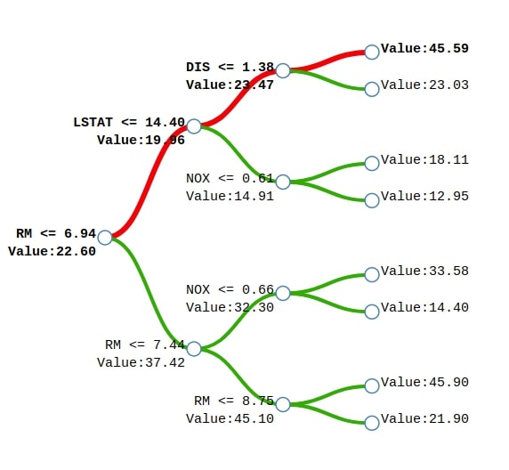
We can notice from the above example of a tree generated for Boston house price prediction. We'll explain how the sample represented by the red line will come to the final prediction. We start with a base price of 22.60 and then subtract 2.64 because the value of feature RM is less than 6.94 to come to the prediction of 19.96. We then add 3.51 to 19.96 to come to the prediction of 23.47 because the value of the feature LSTAT is less than 14.40 in the sample. We'll then add 22.12 to previous prediction 23.47 to come to final prediction 45.59 because the value of feature DIS is less than 1.38 in the sample. This way we'll start with a base value of 22.60 and then add values based on feature contributions.
The treeinterpreter takes as input tree-based model and samples and returns the base value for each sample, contributions of each feature into a prediction of each sample, and predictions for each sample. It'll become clear when we'll go through the examples below.
We'll be explaining both classification and regression models through various examples. We'll start by importing the necessary libraries.
import pandas as pd
import numpy as np

import warnings
warnings.filterwarnings("ignore")
Regression
As first, we'll explain the usage of treeinterpreter when solving a regression task.
Load Dataset
We'll be using California housing datasets available from sklearn for explaining the usage of treeinterpreter to explain ML model predictions on datasets whose prediction variable is continuous. Below we have loaded California housing datasets. We have also printed its description which explains the individual features of the dataset. We have even shown the first few samples of the dataset.
from sklearn.datasets import fetch_california_housing

calif_housing = fetch_california_housing()

for line in calif_housing.DESCR.split("\n")[5:22]:
    print(line)

calif_housing_df = pd.DataFrame(data=calif_housing.data, columns=calif_housing.feature_names)
calif_housing_df["Price($)"] = calif_housing.target

calif_housing_df.head()
Below we have divided the dataset into the train (80%) and test (20%) sets. We'll be using this training dataset for training purposes and randomly select a sample from test data to explain model prediction using treeinterpreter.
from sklearn.model_selection import train_test_split

X_calif, Y_calif = calif_housing.data, calif_housing.target

print("Dataset Size : ", X_calif.shape, Y_calif.shape)

X_train_calif, X_test_calif, Y_train_calif, Y_test_calif = train_test_split(X_calif, Y_calif,
                                                                            train_size=0.8,
                                                                            test_size=0.2,
                                                                            random_state=123)

print("Train/Test Size : ", X_train_calif.shape, X_test_calif.shape, Y_train_calif.shape, Y_test_calif.shape)
DecisionTreeRegressor
The first model that we'll fit to train data is DecisionTreeRegressor as explained below. We have then printed the R2 score of the model on train and test dataset both.
from sklearn.tree import DecisionTreeRegressor

dtree_reg = DecisionTreeRegressor(max_depth=10)
dtree_reg.fit(X_train_calif, Y_train_calif)
print("Test  R^2 Score : %.2f"%dtree_reg.score(X_test_calif, Y_test_calif))
print("Train R^2 Score : %.2f"%dtree_reg.score(X_train_calif, Y_train_calif))
We'll start by loading treeinterpreter. The treeinterpreter has a single method named predict() which takes as input model instance and dataset for which we need explanations. It returns three arrays as output.
- The first array is predictions for a number of samples passed to the method.
- The second array is bias or base value for each sample of data to which individual feature contribution will be added to generate a final prediction.
- The third array is of size (#samples x #no_of_features) as it has the contribution of each feature for each sample which gets added to base/bias value to generate predictions.
Below we have passed the decision tree regressor and California testing dataset to predict() method of treeinterpreter to generate predictions, biases, and feature contributions.
from treeinterpreter import treeinterpreter as ti

preds, bias, contributions = ti.predict(dtree_reg, X_test_calif)
preds.shape, bias.shape, contributions.shape
Below we are explaining various values of output for the 0th sample. We are also adding contributions for the 0th sample to 0th bias value to generate a prediction.
print("Bias For Sample 0                        : %.2f"%bias[0])
print("Constributions For Sample 0              : %s"%contributions[0])
print("Prediction Based on Bias & Contributions : %.2f"%(bias[0] + contributions[0].sum()))
print("Actual Target Value                      : %.2f"%Y_test_calif[0])
print("Target Value As Per Treeinterpreter      : %.2f"%preds[0][0])
Below we are taking a random sample from the test dataset. We have created a method named create_contrbutions_df() which takes as input contributions, sample data, and feature names as input and generates a pandas dataframe where each row represents contributions from each feature. The first row is a bias/base value and the last row has actual prediction calculated by adding all feature contributions to the base/bias value.
import random

random_sample = random.randint(1, len(X_test_calif))
print("Selected Sample     : %d"%random_sample)
print("Actual Target Value : %.2f"%Y_test_calif[random_sample])
print("Predicted Value     : %.2f"%preds[random_sample][0])

def create_contrbutions_df(contributions, random_sample, feature_names):
    contribs = contributions[random_sample].tolist()
    contribs.insert(0, bias[random_sample])
    contribs = np.array(contribs)
    contrib_df = pd.DataFrame(data=contribs, index=["Base"] + feature_names, columns=["Contributions"])
    prediction = contrib_df.Contributions.sum()
    contrib_df.loc["Prediction"] = prediction
    return contrib_df

contrib_df = create_contrbutions_df(contributions, random_sample, calif_housing.feature_names)
contrib_df
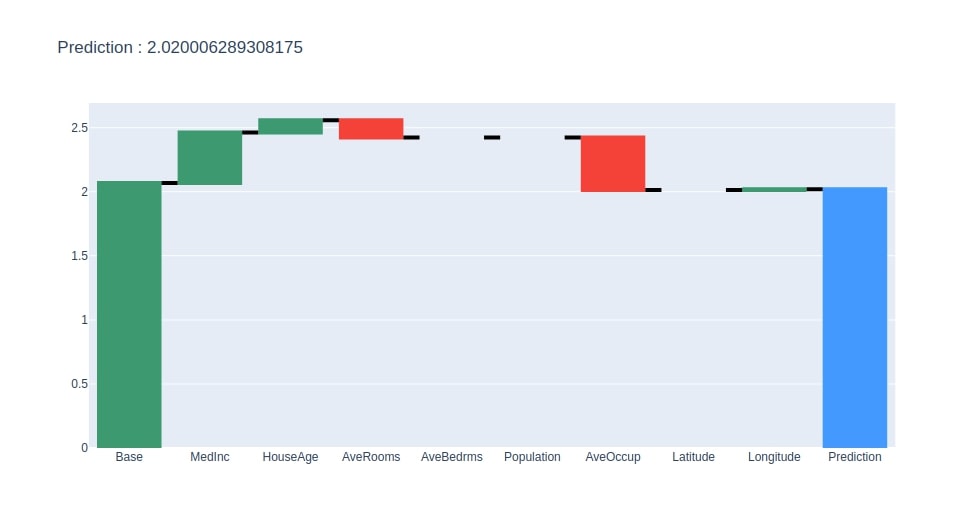
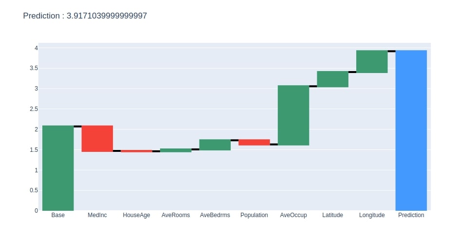
Below we have created a method that takes as input contributions dataframe created earlier and creates a plotly waterfall chart of it. The chart will show how we start with the base value and add contributions of each feature to come for the final prediction.
import plotly.graph_objects as go

def create_waterfall_chart(contrib_df, prediction):
    fig = go.Figure(go.Waterfall(
        name = "Prediction", #orientation = "h",
        measure = ["relative"] * (len(contrib_df)-1) + ["total"],
        x = contrib_df.index,
        y = contrib_df.Contributions,
        connector = {"mode":"between", "line":{"width":4, "color":"rgb(0, 0, 0)", "dash":"solid"}}
    ))

    fig.update_layout(title = "Prediction : %s"%prediction)

    return fig

create_waterfall_chart(contrib_df, contrib_df.loc["Prediction"][0])
ExtraTreeRegressor
The second estimator that we'll use for explaining the usage of treeinterpreter is ExtraTreeRegressor. We'll be following the same process as followed in the first example in all our examples.
Below we have fitted ExtraTreeRegressor to train data and evaluated R2 score on test and train data both. We have also calculated predictions, biases, and feature contributions for the test dataset using treeinterpreter.
from sklearn.tree import ExtraTreeRegressor

etree_reg = ExtraTreeRegressor(max_depth=15)
etree_reg.fit(X_train_calif, Y_train_calif)

print("Test  R^2 Score : %.2f"%etree_reg.score(X_test_calif, Y_test_calif))
print("Train R^2 Score : %.2f"%etree_reg.score(X_train_calif, Y_train_calif))

preds, bias, contributions = ti.predict(etree_reg, X_test_calif)
Below we are generating a contributions dataframe for the random test sample.
random_sample = random.randint(1, len(X_test_calif))
print("Selected Sample     : %d"%random_sample)
print("Actual Target Value : %.2f"%Y_test_calif[random_sample])
print("Predicted Value     : %.2f"%preds[random_sample][0])

contrib_df = create_contrbutions_df(contributions, random_sample, calif_housing.feature_names)
contrib_df
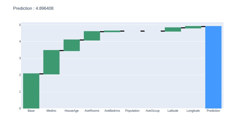
Below we have generated a waterfall chart from the contributions dataframe created in the previous step.
create_waterfall_chart(contrib_df, contrib_df.loc["Prediction"][0])
RandomForestRegressor
The third sklearn estimator that we'll explore is RandomForestRegressor. We have fitted RandomForestRegressor to train data below and evaluated R2 score on test and train data both. We have then generated predictions, biases, and contributions on the test dataset.
from sklearn.ensemble import RandomForestRegressor

rand_forest = RandomForestRegressor()
rand_forest.fit(X_train_calif, Y_train_calif)

print("Test  R^2 Score : %.2f"%rand_forest.score(X_test_calif, Y_test_calif))
print("Train R^2 Score : %.2f"%rand_forest.score(X_train_calif, Y_train_calif))

preds, bias, contributions = ti.predict(rand_forest, X_test_calif)
Below we have generated contributions dataframe for a random sample of test data.
random_sample = random.randint(1, len(X_test_calif))
print("Selected Sample     : %d"%random_sample)
print("Actual Target Value : %.2f"%Y_test_calif[random_sample])
print("Predicted Value     : %.2f"%preds[random_sample][0])

contrib_df = create_contrbutions_df(contributions, random_sample, calif_housing.feature_names)
contrib_df
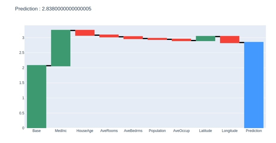
We have now plotted a waterfall chart for the random test sample.
create_waterfall_chart(contrib_df, contrib_df.loc["Prediction"][0])
ExtraTreesRegressor
The last sklearn estimator that we'll explain as a part of the regression task section is ExtraTreesRegressor. Below we have fitted ExtraTreesRegressor to train data and evaluated R2 score on test & train data both. We have then calculated predictions, biases, and feature contributions on test data.
from sklearn.ensemble import ExtraTreesRegressor

etrees_reg = ExtraTreesRegressor()
etrees_reg.fit(X_train_calif, Y_train_calif)

print("Test  R^2 Score : %.2f"%etrees_reg.score(X_test_calif, Y_test_calif))
print("Train R^2 Score : %.2f"%etrees_reg.score(X_train_calif, Y_train_calif))

preds, bias, contributions = ti.predict(etrees_reg, X_test_calif)
Below we have generated contributions dataframe on the random test sample.
random_sample = random.randint(1, len(X_test_calif))
print("Selected Sample     : %d"%random_sample)
print("Actual Target Value : %.2f"%Y_test_calif[random_sample])
print("Predicted Value     : %.2f"%preds[random_sample][0])

contrib_df = create_contrbutions_df(contributions, random_sample, calif_housing.feature_names)
contrib_df
We have then generated a waterfall chart for the contributions dataframe created in the previous step.
create_waterfall_chart(contrib_df, contrib_df.loc["Prediction"][0])
Classification
The second section of this tutorial will explain the usage of treeinterpreter in case of the classification tasks. We'll be using a famous wine classification dataset which is easily available for this. The dataset has information about ingredients used in three different categories of wine. Below, we have loaded the dataset and printed description of individual features as well.
from sklearn.datasets import load_wine

wine = load_wine()

for line in wine.DESCR.split("\n")[5:29]:
    print(line)

wine_df = pd.DataFrame(data=wine.data, columns=wine.feature_names)
wine_df["WineType"] = wine.target

wine_df.head()
We have now divided the dataset into the train (80%) and test (20%) sets.
from sklearn.model_selection import train_test_split

X_wine, Y_wine = wine.data, wine.target

print("Dataset Size : ", X_wine.shape, Y_wine.shape)

X_train_wine, X_test_wine, Y_train_wine, Y_test_wine = train_test_split(X_wine, Y_wine,
                                                                        train_size=0.8,
                                                                        test_size=0.2,
                                                                        stratify=Y_wine,
                                                                        random_state=123)

print("Train/Test Size : ", X_train_wine.shape, X_test_wine.shape, Y_train_wine.shape, Y_test_wine.shape)
DecisionTreeClassifier
The first estimator that we'll try to explain the usage of treeinterpreter for classification task is DecisionTreeClassifier. Below we have trained DecisionTreeClassifier on train data and evaluated the accuracy of the trained model on test and train datasets. We have then generated predictions, biases, and contributions for test samples.
Please make a note of the size of predictions, biases, and contributions this time. They all have the last dimension the same as a number of classes of the target variable.
- The predictions array will have three probabilities, one for each class.
- The biases dataset will have three biases, one for each class.
- The contributions dataset will have three values for each feature, one per each class.
from sklearn.tree import DecisionTreeClassifier

dtree_classif = DecisionTreeClassifier()
dtree_classif.fit(X_train_wine, Y_train_wine)

print("Test  Accuracy : %.2f"%dtree_classif.score(X_test_wine, Y_test_wine))
print("Train Accuracy : %.2f"%dtree_classif.score(X_train_wine, Y_train_wine))

preds, bias, contributions = ti.predict(dtree_classif, X_test_wine)
preds.shape, bias.shape, contributions.shape
Below we have included code that explains the 0th sample of test data. We have also done calculations on how feature contributions are added to biases to generate prediction class.
print("Bias For Sample 0                        : %s"%bias[0])
print("Constributions For Sample 0              : %s"%contributions[0])
print("Prediction Based on Bias & Contributions : %.2f"%np.argmax((bias[0] + contributions[0].sum(axis=0))))
print("Actual Target Value                      : %.2f"%Y_test_wine[0])
print("Target Value As Per Treeinterpreter      : %.2f"%np.argmax(preds[0]))
We have now taken a random sample of test data. We have then created a method named create_contrbutions_df() which takes as input contributions, random sample data, and feature names to generate contributions dataframe like explained during the regression section. The only difference in contributions dataframe this time is that it'll have three columns, one for each class of data.
random_sample = random.randint(1, len(X_test_wine))
print("Selected Sample     : %d"%random_sample)
print("Actual Target Value : %s"%wine.target_names[Y_test_wine[random_sample]])
print("Predicted Value     : %s"%wine.target_names[np.argmax(preds[random_sample])])

def create_contrbutions_df(contributions, random_sample, feature_names):
    contribs = contributions[random_sample].tolist()
    contribs.insert(0, bias[random_sample])
    contribs = np.array(contribs)
    contrib_df = pd.DataFrame(data=contribs, index=["Base"] + feature_names, columns=["Contributions_0", "Contributions_1", "Contributions_2"])
    prediction = contrib_df[["Contributions_0", "Contributions_1", "Contributions_2"]].sum()
    contrib_df.loc["Prediction"] = prediction
    return contrib_df

contrib_df = create_contrbutions_df(contributions, random_sample, wine.feature_names)
contrib_df
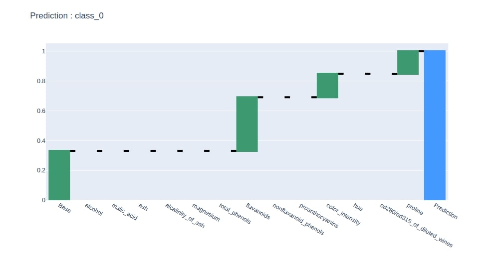
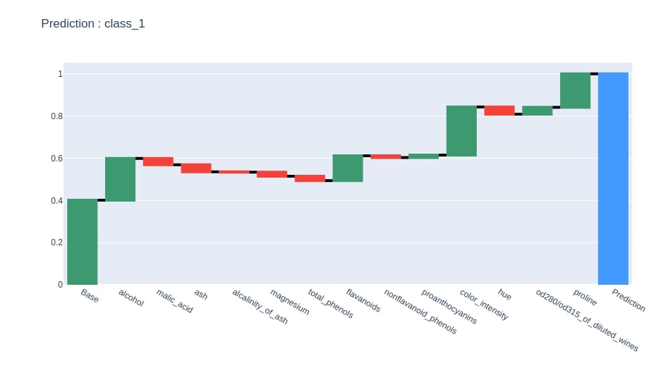
Below we have generated a waterfall chart from the contributions dataframe based on contributions of the column where the last row has value 1.
idx = contrib_df.loc["Prediction"].values.argmax()
col = "Contributions_%d"%idx
contrib_df = contrib_df[[col]].rename(columns={col:"Contributions"})

create_waterfall_chart(contrib_df, wine.target_names[idx])
ExtraTreeClassifier
The second sklearn estimator that we'll train is ExtraTreeClassifier. We have also printed the accuracy of the model on the test and train dataset. We have also then generated predictions, biases, and contributions for this model on the test dataset.
from sklearn.tree import ExtraTreeClassifier

etree_classif = ExtraTreeClassifier()
etree_classif.fit(X_train_wine, Y_train_wine)

print("Test  Accuracy : %.2f"%etree_classif.score(X_test_wine, Y_test_wine))
print("Train Accuracy : %.2f"%etree_classif.score(X_train_wine, Y_train_wine))

preds, bias, contributions = ti.predict(etree_classif, X_test_wine)
Below we have generated contributions dataframe for a random sample of the test dataset.
random_sample = random.randint(1, len(X_test_wine))
print("Selected Sample     : %d"%random_sample)
print("Actual Target Value : %s"%wine.target_names[Y_test_wine[random_sample]])
print("Predicted Value     : %s"%wine.target_names[np.argmax(preds[random_sample])])

contrib_df = create_contrbutions_df(contributions, random_sample, wine.feature_names)
contrib_df
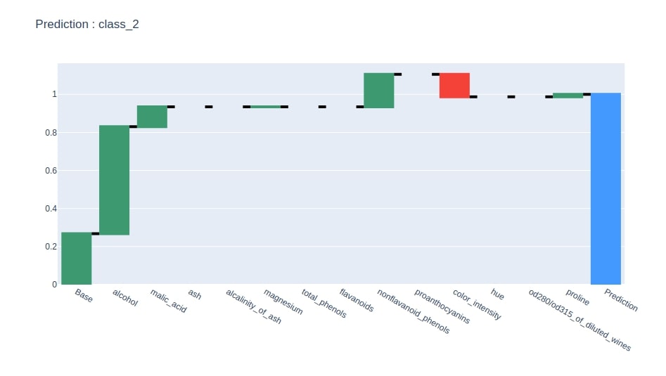
We have now generated a waterfall chart from the contributions dataframe using column where the last row is 1.
idx = contrib_df.loc["Prediction"].values.argmax()
col = "Contributions_%d"%idx
contrib_df = contrib_df[[col]].rename(columns={col:"Contributions"})

create_waterfall_chart(contrib_df, wine.target_names[idx])
RandomForestClassifier
The third estimator that we have trained on wine train data is RandomForestClassifier. We have also printed the test and train the accuracy of the model. We then calculated predictions, biases, and feature contributions for test samples.
from sklearn.ensemble import RandomForestClassifier

rf_classif = RandomForestClassifier()
rf_classif.fit(X_train_wine, Y_train_wine)

print("Test  Accuracy : %.2f"%rf_classif.score(X_test_wine, Y_test_wine))
print("Train Accuracy : %.2f"%rf_classif.score(X_train_wine, Y_train_wine))

preds, bias, contributions = ti.predict(rf_classif, X_test_wine)
We have now taken a random test sample and generated a contributions dataframe based on it.
random_sample = random.randint(1, len(X_test_wine))
print("Selected Sample     : %d"%random_sample)
print("Actual Target Value : %s"%wine.target_names[Y_test_wine[random_sample]])
print("Predicted Value     : %s"%wine.target_names[np.argmax(preds[random_sample])])

contrib_df = create_contrbutions_df(contributions, random_sample, wine.feature_names)
contrib_df
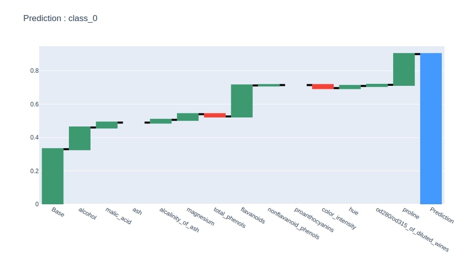
Below we have plotted a waterfall chart of predicted class feature contributions.
idx = contrib_df.loc["Prediction"].values.argmax()
col = "Contributions_%d"%idx
contrib_df = contrib_df[[col]].rename(columns={col:"Contributions"})

create_waterfall_chart(contrib_df, wine.target_names[idx])
ExtraTreesClassifier
The fourth and last estimator that we'll explain is ExtraTreesClassifier. We have trained ExtraTreesClassifier on train data and calculated accuracy on test and train data. We have then calculated predictions, biases, and feature contributions using treeinterpreter for test samples.
from sklearn.ensemble import ExtraTreesClassifier

etrees_classif = ExtraTreesClassifier()
etrees_classif.fit(X_train_wine, Y_train_wine)

print("Test  Accuracy : %.2f"%etrees_classif.score(X_test_wine, Y_test_wine))
print("Train Accuracy : %.2f"%etrees_classif.score(X_train_wine, Y_train_wine))

preds, bias, contributions = ti.predict(etrees_classif, X_test_wine)
Below we have taken a random sample from test data and generated feature contributions dataframe from it.
random_sample = random.randint(1, len(X_test_wine))
print("Selected Sample     : %d"%random_sample)
print("Actual Target Value : %s"%wine.target_names[Y_test_wine[random_sample]])
print("Predicted Value     : %s"%wine.target_names[np.argmax(preds[random_sample])])

contrib_df = create_contrbutions_df(contributions, random_sample, wine.feature_names)
contrib_df
At last, we have generated a waterfall chart for predicted class feature contributions from the contributions dataframe created in the previous step.
idx = contrib_df.loc["Prediction"].values.argmax()
col = "Contributions_%d"%idx
contrib_df = contrib_df[[col]].rename(columns={col:"Contributions"})

create_waterfall_chart(contrib_df, wine.target_names[idx])
Text Classification Example
We'll now explain how we can use treeinterpreter with a text dataset which is trained using tree based classifier. We'll start by downloading the spam/ham mails dataset from the UCI machine learning datasets repository.
!wget https://archive.ics.uci.edu/ml/machine-learning-databases/00228/smsspamcollection.zip
!unzip smsspamcollection.zip
Below we have loaded the dataset as a list of text mails and their class (ham/spam).
with open('SMSSpamCollection') as f:
    data = [line.strip().split('\t') for line in f.readlines()]

y, text = zip(*data)
import collections

collections.Counter(y)
We have divided the dataset below into train (75%) and test (25%) sets.
from sklearn.model_selection import train_test_split

text_train, text_test, y_train, y_test = train_test_split(text, y,
                                                          random_state=42,
                                                          test_size=0.25,
                                                          stratify=y)
Below we have used the TF-IDF vectorizer to convert text data to the floating matrix. We have then trained the RandomForestClassifier classifier on this transformed matrix and printed test & train accuracy. We have then calculated predictions, biases, and contributions of test samples using treeinterpreter.
If you don’t have a background on feature extraction from text data and interested in learning about the same then please feel free to check our tutorial on the same.
from sklearn.feature_extraction.text import TfidfVectorizer
from sklearn.ensemble import RandomForestClassifier
from sklearn.metrics import confusion_matrix, classification_report

tfidf_vectorizer = TfidfVectorizer(stop_words="english", max_features=500)
tfidf_vectorizer.fit(text_train)

X_train_tfidf = tfidf_vectorizer.transform(text_train)
X_test_tfidf = tfidf_vectorizer.transform(text_test)


print(X_train_tfidf.shape, X_test_tfidf.shape)

rf = RandomForestClassifier()

rf.fit(X_train_tfidf, y_train)

print("Test  Accuracy : %.2f"%rf.score(X_test_tfidf, y_test))
print("Train Accuracy : %.2f"%rf.score(X_train_tfidf, y_train))

preds, bias, contributions = ti.predict(rf, X_test_tfidf)
preds.shape, bias.shape, contributions.shape
Below we have taken a random test sample and generated a contributions dataframe based on words that contribute to prediction. We have kept a dataframe with only 20 important features as main contributors.
random_sample = random.randint(1, len(text_test))
print("Selected Sample     : %d"%random_sample)
print("Actual Target Value : %s"%y_test[random_sample])
print("Predicted Value     : %s"%["ham", "spam"][np.argmax(preds[random_sample])])
print("Test Sample : ", text_test[random_sample])

contribs = contributions[random_sample].tolist()
contribs.insert(0, bias[random_sample])
contribs = np.array(contribs)
contrib_df = pd.DataFrame(data=contribs, index=["Base"] + tfidf_vectorizer.get_feature_names(), columns=["ham", "spam"])
prediction = contrib_df[["ham", "spam"]].sum()
contrib_df.loc["Prediction"] = prediction

first = pd.DataFrame(contrib_df.loc["Base"]).T
contrib_df = contrib_df[1:].sort_values(by=y_test[random_sample])[-20:]
contrib_df = pd.concat((first,contrib_df))
contrib_df
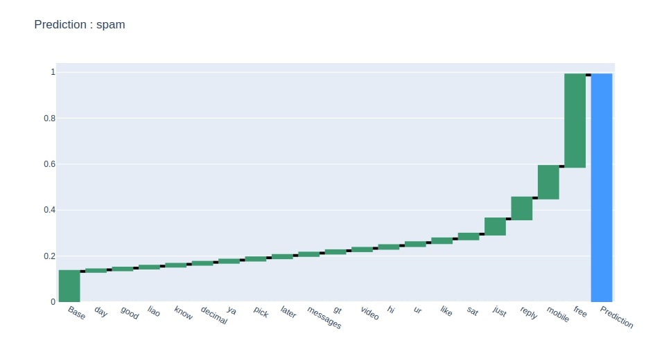
Below we have generated a waterfall chart showing 20 main features that contributed most to prediction.
pred = y_test[random_sample]
create_waterfall_chart(contrib_df[[pred]].rename(columns={pred:"Contributions"}), pred)
References
- Treeinterpreter Explanation
- Feature Extraction From Text Data using Scikit-Learn
- SHAP - Explain Machine Learning Model Predictions using Game Theoretic Approach
- How to Use LIME to Understand sklearn Models Predictions?
- How to Use eli5 to Understand sklearn Models, their Performance, and their Predictions?
- Yellowbrick - Visualize Sklearn's Classification & Regression Metrics in Python
- interpret-text - Interpret NLP Models and Their Predictions
- dice-ml - Diverse Counterfactual Explanations for ML Models
- interpret-ml - Explain Machine Learning Models and Their Predictions
- Yellowbrick - Text Data Visualizations
 Sunny Solanki
Sunny Solanki
Intro: Software Developer | Youtuber | Bonsai Enthusiast
About: Sunny Solanki holds a bachelor's degree in Information Technology (2006-2010) from L.D. College of Engineering. Post completion of his graduation, he has 8.5+ years of experience (2011-2019) in the IT Industry (TCS). His IT experience involves working on Python & Java Projects with US/Canada banking clients. Since 2020, he’s primarily concentrating on growing CoderzColumn.
His main areas of interest are AI, Machine Learning, Data Visualization, and Concurrent Programming. He has good hands-on with Python and its ecosystem libraries.
Apart from his tech life, he prefers reading biographies and autobiographies. And yes, he spends his leisure time taking care of his plants and a few pre-Bonsai trees.
Contact: sunny.2309@yahoo.in


![YouTube Subscribe]() Comfortable Learning through Video Tutorials?
Comfortable Learning through Video Tutorials?
If you are more comfortable learning through video tutorials then we would recommend that you subscribe to our YouTube channel.
![Need Help]() Stuck Somewhere? Need Help with Coding? Have Doubts About the Topic/Code?
Stuck Somewhere? Need Help with Coding? Have Doubts About the Topic/Code?
 Stuck Somewhere? Need Help with Coding? Have Doubts About the Topic/Code?
When going through coding examples, it's quite common to have doubts and errors.
If you have doubts about some code examples or are stuck somewhere when trying our code, send us an email at coderzcolumn07@gmail.com. We'll help you or point you in the direction where you can find a solution to your problem.
You can even send us a mail if you are trying something new and need guidance regarding coding. We'll try to respond as soon as possible.
![Share Views]() Want to Share Your Views? Have Any Suggestions?
Want to Share Your Views? Have Any Suggestions?
 Want to Share Your Views? Have Any Suggestions?
If you want to
- provide some suggestions on topic
- share your views
- include some details in tutorial
- suggest some new topics on which we should create tutorials/blogs
 treeinterpreter, tree-models