How to Display Rich Media Contents (Image, Audio, Video, etc) in Jupyter Notebook?
Jupyter notebook and Lab have become a favorite tool for data scientists and developers all over the world to perform data analysis and related tasks.
> Why Jupyter Notebooks are Famous? Why Jupyter Notebooks are Preferred tool by Data Scientists Worldwide?
Its user-friendly interface and out-of-box functionalities like supporting shell commands from the notebook make it a unique and go-to tool in the data science community.
The jupyter notebook is based on the IPython kernel running under the hood. IPython kernel is just like a normal python interpreter but with lots of additional functionalities.
As Jupyter notebook is used by the majority of data scientists worldwide, it supports displaying rich media contents (image, markdown, latex, video, audio, HTML, etc.). This frees users from the hassle of using different tools to see contents of different types. We can play audio and video in notebook which is displayed.
It even let us include static and interactive charts in notebooks that are created during analysis. It even let us create dashboards (voila).
All pieces of analysis are available in one place. This makes reproducible research easy to conduct.
It is also very useful for presentation purposes as many people use Jupyter Notebooks for presentations as well.
All these benefits make Jupyter notebooks the most preferred tool by data scientists worldwide.
> How can we display Rich Media Contents in Notebooks?
IPython kernel that power Jupyter notebook has a module named 'display' that provides us with a list of classes and methods that can be used to display rich media contents of different types in Jupyter notebook and Jupyter Lab.
> What Can You Learn From This Article?
As a part of this tutorial, we have explained how to display Rich media contents/outputs in Jupyter Notebook. This includes contents like audio/sound, video, latex, markdown, HTML, iframe, SVG, pdf, etc. The functions and classes to display rich outputs are available through "IPython.display" which we have listed in our first section below.
Below, we have listed important sections of tutorial to give an overview of material covered.
Important Sections Of Tutorial
- Important Classes and Functions of "IPython.display" Module
- How to Display "Audio" or "Sound" Player in Jupyter Notebook?
- How to Display "Code" in Jupyter Notebook?
- How to Display File as Downloadable Link using "FileLink" in Jupyter Notebook?
- How to Display All Files in Directory as Downloadable Links using "FileLinks" in Jupyter Notebook?
- How to Display "HTML" in Jupyter Notebook?
- How to Display "IFrame" in Jupyter Notebook?
- How to Display "Images" in Jupyter Notebook?
- How to Display "SVG Images" in Jupyter Notebook?
- How to Display "JSON" in Jupyter Notebook?
- How to Display "Javascript" in Jupyter Notebook?
- How to Display "Markdown" in Jupyter Notebook?
- How to Display Mathematical Formulas using "LaTex" in Jupyter Notebook?
- How to Display "Scribd Documents" in Jupyter Notebook?
- How to Print Formatted Output using "Pretty Print" in Jupyter Notebook?
- How to Display "Videos" in Jupyter Notebook?
- How to Display "YouTube Videos" in Jupyter Notebook?
- How to Display "Vimeo Videos" in Jupyter Notebook?
- How to Combine Rich Media Contents Of Different Types (Audio, Video, Image, Code, Latex, Markdown, etc) and Display them in Jupyter Notebook using "display()"?
1. Important Classes and Functions of "IPython.display" Module 
Below is a list of classes and methods available with the IPython.display module.
Classes
The classes displayed below accept data of a particular type and when executed from the jupyter notebook cell will display the content of that type in a notebook.
- Audio
- Code
- FileLink
- FileLinks
- HTML
- IFrame
- Image
- SVG
- JSON
- JavaScript
- Markdown
- Latex
- ScribdDocument
- Pretty
- Video
- YouTubeVideo
- VimeoVideo
Functions
The "display_*()" functions can take as input many objects created using classes mentioned above and display all of them one after another. The method as per their name takes objects of one kind as input except for the last display() method which can combine contents of different types and display them.
- display_html()
- display_jpeg()
- display_png()
- display_svg()
- display_json()
- display_javascript()
- display_markdown()
- display_latex()
- display_pretty()
- display()
This ends small introduction and now let's start with coding part. We'll start by importing the display module.
from IPython import display
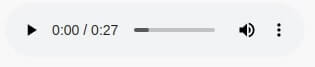
2. How to Display "Audio" or "Sound" Player in Jupyter Notebook? 
The Audio class let us display audio files in a jupyter notebook. It provides us with a simple player that we can pause/play to listen to the audio. The first argument of the method is data which accepts one of the below inputs and generates an Audio object which when displayed will display a small player that can play audio.
- numpy array (1d or 2d) of a waveform
- list of floats containing waveform
- local audio filename
- URL
Below we have given as input URL of an audio file and it'll display an audio object which can play that audio. We have also explained below with examples of how we can play audio from local files. We can also set the autoplay parameter to True and it'll start playing audio immediately. It has another important parameter named rate which specifies sampling rate and should be used if data is provided as a numpy array or list of floats.
When we give an object created by any class as the last line in the notebook cell, it'll display an object of that type.
Please make a note that the majority of classes available from the display module provides boolean parameter named embed which if set to True will put DATA URI of the content into a notebook and next time we won't need to load that content into the notebook from file/URL.
display.Audio(url="https://file-examples-com.github.io/uploads/2017/11/file_example_MP3_700KB.mp3")
display.Audio(filename="sample_audio.mp3")
display.Audio(data="sample_wav.wav")

display.Audio(data="sample_wav.wav", autoplay=True)
3. How to Display "Code" in Jupyter Notebook? 
The Code class can be used to display code in syntax-highlighted format. We can provide code information to the class in one of the below-mentioned ways.
- String of code
- Local filename
- URL where the file resides
Below we have explained with simple examples of how we can use this class.
display.Code("profiling_examples/example1_modified.py")
display.Code(filename = "sample.js")
4. How to Display File as Downloadable Link using "FileLink" in Jupyter Notebook? 
The FileLink class lets us create links around files on local. It accepts a file name as input and will create a link around it. We can give prefix and suffix to use around link using result_html_prefix and result_html_suffix commands.
We have explained the usage of the class below with simple examples. This can be useful when we are running a notebook on platforms like kaggle or google collab or any other platform where we don't have access to local disks to download files which might be generated during our analysis like model weights file, plotting files, etc.
display.FileLink(path="profiling_examples/example1_modified.py")

display.FileLink(path="profiling_examples/example1_modified.py", result_html_prefix="Profiling Examples : ")

display.FileLink(path="profiling_examples/example1_modified.py", result_html_prefix="Profiling Examples : ", result_html_suffix=" Sample Profiling File")

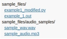
5. How to Display All Files in Directory as Downloadable Links using "FileLinks" in Jupyter Notebook? 
The FileLinks class works exactly like the FileLink class with the only difference that it accepts directory names as input and creates a list of links for all the files present in it.
Below we have explained the usage of the same on a temporary folder named sample_files which we created for this. It also provides a boolean parameter named recursive which is True by default and recurses in all subdirectories to display files in all of them. We can set this parameter to False if we don't want links of subdirectories.
display.FileLinks(path="sample_files")
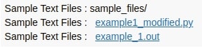
display.FileLinks(path="sample_files", result_html_prefix="Sample Text Files : ", recursive=False)
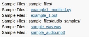
display.FileLinks(path="sample_files", result_html_prefix="Sample Files : ", recursive=True)
6. How to Display "HTML" in Jupyter Notebook? 
The HTML class let us display HTML in notebook. The class accepts a list of the below-mentioned data types as input to create an HTML object.
- String containing HTML code
- URL
- HTML File on local system
Below we have explained the usage of the class with simple examples. We have also created a sample HTML file from one of our blogs and displayed it as a sample.
sample_html = '<html><body><h3>Hello World</h3><h4>Hello World</h4><h5>Hello World</h5><h6>Hello World</h6></body></html>'
display.HTML(data=sample_html)
display.HTML(url="https://google.com")
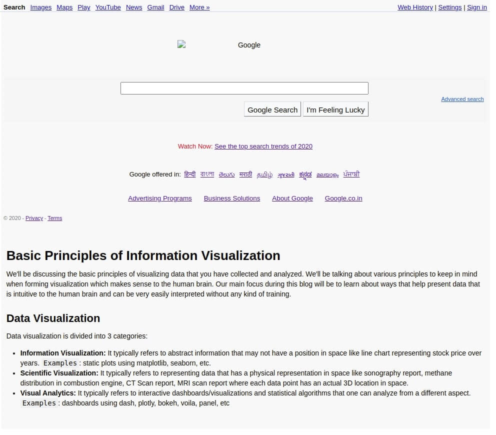
display.HTML(filename="basic-principles-of-information-visualization.html")
Basic Principles of Information Visualization
We'll be discussing the basic principles of visualizing data that you have collected and analyzed. We'll be talking about various principles to keep in mind when forming visualization which makes sense to the human brain. Our main focus during this blog will be to learn about ways that help present data that is intuitive to the human brain and can be very easily interpreted without any kind of training.
Data Visualization
Data visualization is divided into 3 categories:
- Information Visualization: It typically refers to abstract information that may not have a position in space like line chart representing stock price over years.
Examples: static plots using matplotlib, seaborn, etc. - Scientific Visualization: It typically refers to representing data that has a physical representation in space like sonography report, methane distribution in combustion engine, CT Scan report, MRI scan report where each data point has an actual 3D location in space.
- Visual Analytics: It typically refers to interactive dashboards/visualizations and statistical algorithms that one can analyze from a different aspect.
Examples: dashboards using dash, plotly, bokeh, voila, panel, etc
"display_html()"
The display_html() method takes as input list of HTML object created using display.HTML class and displays all of them one after another in jupyter notebook. Below we have explained the usage with a simple example where we combine HTML of google URL and local file.
html1 = display.HTML(url="https://google.com")
html2 = display.HTML(filename="basic-principles-of-information-visualization.html")
display.display_html(html1, html2)
7. How to Display "IFrame" in Jupyter Notebook? 
The IFrame class lets us display iframes in jupyter notebooks. It lets us also specify the width and height of the iframe. Below we have used an iframe to display local HTML files and IPython docs using URL.
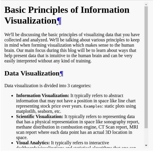
display.IFrame(src="basic-principles-of-information-visualization.html", width=500, height=500)
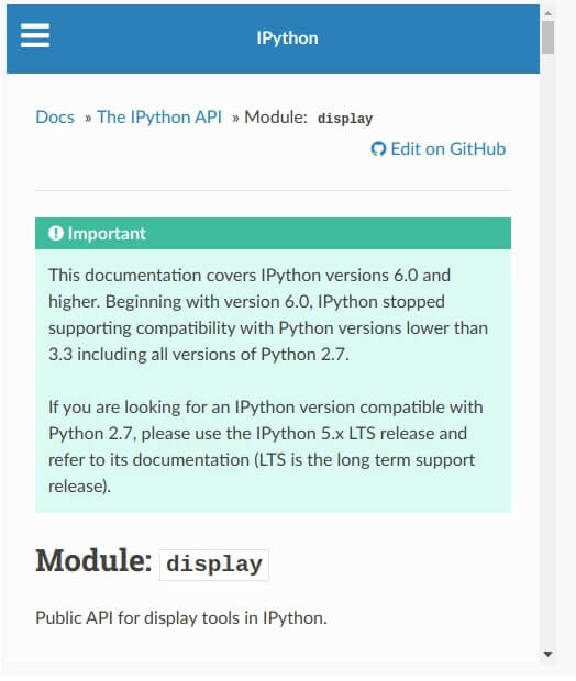
display.IFrame(src="https://ipython.readthedocs.io/en/stable/api/generated/IPython.display.html", width=500, height=600)
8. How to Display "Images" in Jupyter Notebook? 
The Image class let us display image of type jpg/jpeg/png/gif in jupyter notebook. We can give either image information as str/bytes or filename/URL. Below we have explained with a few simple examples of how we can display images of different types loaded from local file and URL.
display.Image("cc2.png", height=150, width=150)

display.Image("https://storage.googleapis.com/coderzcolumn/static/blogs/home/home_main.jpg")

img_data = open("cc2.png", "rb").read()
display.Image(data=bytearray(img_data), height=150, width=150)
display_jpeg()
The display_jpeg() method takes as input image objects of jpeg/jpg files created using the Image class and display images one after another in a notebook.
img2 = display.Image("https://storage.googleapis.com/coderzcolumn/static/blogs/home/home_main.jpg")
display.display_jpeg(img2)
display_png()
The display_png() method works like the display_jpeg() method and takes as input a list of image objects containing information about the list of png files.
img1 = display.Image("cc2.png", height=150, width=150)
display.display_png(img1)
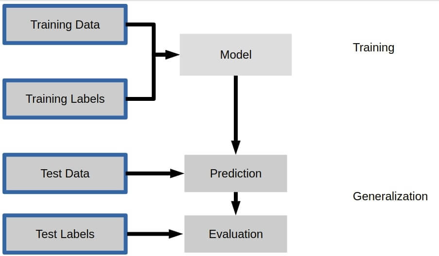
9. How to Display "SVG Images" in Jupyter Notebook? 
The SVG class lets us display the SVG images in a jupyter notebook. We can provide the file name of the image on a local system or web URL to display the SVG image.
display.SVG(filename="supervised_workflow.svg")
display_svg()
The display_svg() image takes as an input list of SVG objects created using the SVG class and displays them one after another.
img = display.SVG("supervised_workflow.svg")
display.display_svg(img)
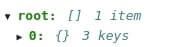
10. How to Display "JSON" in Jupyter Notebook? 
The JSON class displays contents of json as a directory-like structure in jupyter notebook which we can explore by expanding/collapsing node of structure. We need to give json dictionary as input to the method and it'll display contents in a tree-like interactive structure. The class can load JSON from the local files as well as URLs on the web.
Please make a note that this functionality only works with Jupyter lab. It does not work in a jupyter notebook at the time of writing this article.
json_data = [{ "Name": "William", "Employee ID" : 1, "Address": "New York"}]
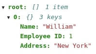
display.JSON(data=json_data)
display.JSON(data=json_data, expanded=True)
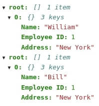
display_json()
The display_json() method takes as input a bunch of json objects created using JSON class and displays all of them one after another.
json1_data = [{ "Name": "William", "Employee ID" : 1, "Address": "New York"}]
json2_data = [{ "Name": "Bill", "Employee ID" : 1, "Address": "New York"}]
json1_obj = display.JSON(json1_data, expanded=True)
json2_obj = display.JSON(json2_data, expanded=True)
display.display_json(json1_obj, json2_obj)
11. How to Display "Javascript" in Jupyter Notebook? 
The Javascript class lets us execute javascript code in jupyter notebook. We can provide the file name or URL of javascript code and it'll execute it. We can access the HTML element of cell output using the element variable in javascript and modify it according to our need to display the output of script execution in the cell output of the notebook. Below we have executed a simple javascript that compares three numbers and prints the largest number as cell output by setting the innerHTML attribute of element.
Please make a note that this functionality only works with Jupyter lab. It does not work in a jupyter notebook at the time of writing this article.
sample.js
// program to find the largest among three numbers
// take input from the user
const num1 = 12
const num2 = 10
const num3 = 35
let largest;
// check the condition
if(num1 >= num2 && num1 >= num3) {
largest = num1;
}
else if (num2 >= num1 && num2 >= num3) {
largest = num2;
}
else {
largest = num3;
}
// display the result
element.innerHTML = '<h1>Hello World</h1>'
display.Javascript(filename="sample.js")

display_javascript()
The display_javascript() method takes as input list of objects created using Javascript class and executes all of them one after another.
jscript1 = display.Javascript(filename="sample.js")
display.display_javascript(jscript1)
12. How to Display "Markdown" in Jupyter Notebook? 
The Markdown class let us display markdown in jupyter notebook. Jupyter notebook itself provides markdown cells already where we can display markdowns but this class can be useful when we are getting markdown data from a different sources in code. Below we have explained with a simple example of how we can use it. The class can also load markdown from a file on local or URL on the web.
If you are interested in learning about markdown then please visit the below link.
markdown = '''
# H1 Heading
## H2 Heading
* L1
* L2
**Bold Text**
'''
display.Markdown(markdown)
display_markdown()
The display_markdown() method accepts a bunch of markdown objects created using the Markdown class and displays all of them one after another.
m1 = '''
# H1 Heading
## H2 Heading
'''
m2 = '''
* L1
* L2
'''
m3 = '''
**Bold Text**
'''
m1_obj = display.Markdown(m1)
m2_obj = display.Markdown(m2)
m3_obj = display.Markdown(m3)
display.display_markdown(m1_obj, m3_obj, m2_obj)
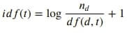
13. How to Display Mathematical Formulas using "LaTex" in Jupyter Notebook? 
The Latex class let us display latex in a jupyter notebook which is generally used to display mathematical formula in a jupyter notebook. The jupyter notebook uses mathjax javascript to display latex in the jupyter notebook. We can provide latex data as string or file name or URL on the web to class. Below we have explained with a simple example of how we can display formula in a jupyter notebook which can be a requirement of many scientific projects.
If you are interested in learning about latex then please visit the below link.
idf = '''
$
idf(t) = {\log_{} \dfrac {n_d} {df(d,t)}} + 1
$
'''
display.Latex(idf)
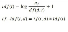
display_latex()
The display_latex() takes as an input list of Latex objects and displays latex in all of them one after another.
idf = '''
$
idf(t) = {\log_{} \dfrac {n_d} {df(d,t)}} + 1
$
'''
tf_idf = '''
$
tf{-}idf(t,d) = tf(t,d) * idf(t)
$
'''
idf_latex = display.Latex(idf)
tf_idf_latex = display.Latex(tf_idf)
display.display_latex(idf_latex, tf_idf_latex)
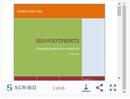
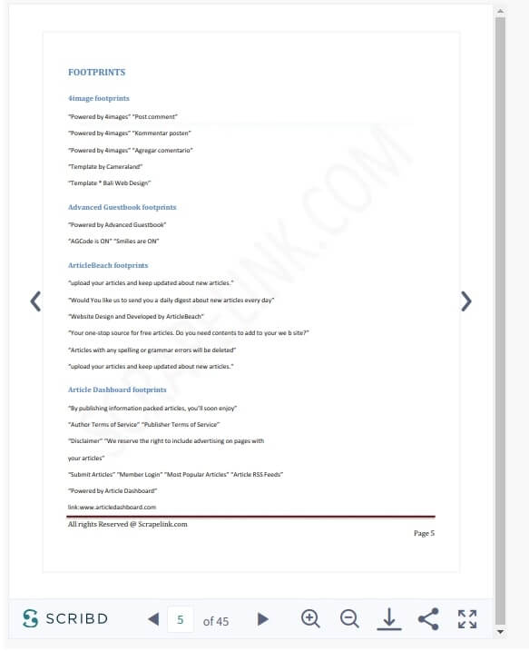
14. How to Display "Scribd Documents" in Jupyter Notebook? 
The ScribdDocument class lets us display Scribd pdf files in a jupyter notebook. We need to provide the unique id of the book on Scribd and it'll display a document in a notebook which we can then read. We can also specify the height and width of the frame which will display the book. It even let us specify the starting page number using the start_page parameter in order to start reading from that page.
Below we have shown the notebook available from the below URL.
display.ScribdDocument("201731015", width=400, height=300)
display.ScribdDocument("201731015", width=550, height=700, start_page=5, view_mode="book")
15. How to Print Formatted Output using "Pretty Print" in Jupyter Notebook? 
The Pretty class lets us display contents of file/URL or string in pretty format.
display.Pretty("profiling_examples/example1_modified.py")
display_pretty()
The display_pretty() method accepts a list of Pretty objects and displays all one after another.
pretty1 = '''
from memory_profiler import profile

@profile(precision=4)
def main_func():
    import random
    arr1 = [random.randint(1,10) for i in range(100000)]
    arr2 = [random.randint(1,10) for i in range(100000)]
    arr3 = [arr1[i]+arr2[i] for i in range(100000)]
    tot = sum(arr3)
    print(tot)

if __name__ == "__main__":
    main_func()
'''
pretty1_obj = display.Pretty(pretty1)
display.display_pretty(pretty1_obj)
16. How to Display "Videos" in Jupyter Notebook? 
The Video class let us display and play video in a jupyter notebook. We can provide either file on local or a URL on the web from where to display the video. We can also provide video data as str or bytes and it'll create a video out of it and display it in a notebook. We have below explained how we can play video from URL and local file.
display.Video("https://file-examples-com.github.io/uploads/2017/04/file_example_MP4_480_1_5MG.mp4")

display.Video("file_example_MP4_480_1_5MG.mp4")
17. How to Display "YouTube Videos" in Jupyter Notebook? 
The YouTubeVideo class let us display and play youtube videos in a jupyter notebook. We need to provide an ID of the video and it'll embed the video in the jupyter notebook. We can then watch it in the notebook. We can also specify the starting position of the video and it'll play from that second.
display.YouTubeVideo(id="OfIQW6s1-ew", width=400, height=300)
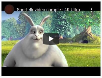
display.YouTubeVideo(id="OfIQW6s1-ew", width=400, height=300, start=15)

18. How to Display "Vimeo Videos" in Jupyter Notebook? 
The VimeoVideo class let us watch Vimeo videos in a jupyter notebook. We need to provide an ID of the video in order to view it.
display.VimeoVideo(id=253989945, width=400, height=300,)

19. How to Combine Rich Media Contents Of Different Types (Audio, Video, Image, Code, Latex, Markdown, etc) and Display them in Jupyter Notebook using "display()"? 
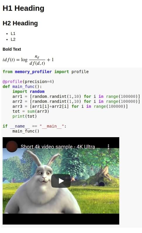
The display() method can take as input objects created using any of the classes mentioned above and will display all of them one after another. This method can be used to combine the contents of different types to display all of them together in a notebook.
Below we have explained with a simple example of how we can combine markdown, latex, code, and video objects in order to display all of them together in one cell output.
markdown = '''
# H1 Heading
## H2 Heading

* L1
* L2

**Bold Text**
'''

idf = '''
$
idf(t)  = {\log_{} \dfrac {n_d} {df(d,t)}} + 1
$
'''

idf_obj = display.Latex(idf)

markdown_obj = display.Markdown(markdown)

code_obj = display.Code("profiling_examples/example1_modified.py")

video_obj = display.YouTubeVideo(id="OfIQW6s1-ew", width=400, height=300)

display.display(markdown_obj, idf_obj, code_obj, video_obj)
This ends our small tutorial explaining how we can use the IPython.display module to display RICH Media outputs of different types in jupyter notebook.
References
 Sunny Solanki
Sunny Solanki
Intro: Software Developer | Youtuber | Bonsai Enthusiast
About: Sunny Solanki holds a bachelor's degree in Information Technology (2006-2010) from L.D. College of Engineering. Post completion of his graduation, he has 8.5+ years of experience (2011-2019) in the IT Industry (TCS). His IT experience involves working on Python & Java Projects with US/Canada banking clients. Since 2020, he’s primarily concentrating on growing CoderzColumn.
His main areas of interest are AI, Machine Learning, Data Visualization, and Concurrent Programming. He has good hands-on with Python and its ecosystem libraries.
Apart from his tech life, he prefers reading biographies and autobiographies. And yes, he spends his leisure time taking care of his plants and a few pre-Bonsai trees.
Contact: sunny.2309@yahoo.in


![YouTube Subscribe]() Comfortable Learning through Video Tutorials?
Comfortable Learning through Video Tutorials?
If you are more comfortable learning through video tutorials then we would recommend that you subscribe to our YouTube channel.
![Need Help]() Stuck Somewhere? Need Help with Coding? Have Doubts About the Topic/Code?
Stuck Somewhere? Need Help with Coding? Have Doubts About the Topic/Code?
 Stuck Somewhere? Need Help with Coding? Have Doubts About the Topic/Code?
When going through coding examples, it's quite common to have doubts and errors.
If you have doubts about some code examples or are stuck somewhere when trying our code, send us an email at coderzcolumn07@gmail.com. We'll help you or point you in the direction where you can find a solution to your problem.
You can even send us a mail if you are trying something new and need guidance regarding coding. We'll try to respond as soon as possible.
![Share Views]() Want to Share Your Views? Have Any Suggestions?
Want to Share Your Views? Have Any Suggestions?
 Want to Share Your Views? Have Any Suggestions?
If you want to
- provide some suggestions on topic
- share your views
- include some details in tutorial
- suggest some new topics on which we should create tutorials/blogs
 jupyter-notebook, content-display