Optax: Learning Rate Schedules for Flax (JAX) Networks
JAX is a deep learning research framework recently introduced by Google and is written in Python. It provides functionalities like numpy-like API on CPU/GPU/TPU, automatic gradients, just-in-time compilation, etc. It's commonly used in many Google projects for deep learning research. JAX is a low-level library just like Tensorflow which can require many lines of code to design a network. To solve this, Google researchers designed another library named Flax on top of JAX to simplify the design of neural networks. Flax let us create neural networks just like we do with PyTorch.
Initially, Flax had its own sub-module of optimizers (SGD, Adam, etc.). But another team at Google designed a package named Optax which has implemented the majority of optimizers that are commonly used in deep learning nowadays. Due to this, Flax team has deprecated their sub-module of optimizers and recommends to everyone that we use optimizers available from Optax.
Generally, when we train a neural network using optimizers like Stochastic Gradient Descent, it keeps the learning rate the same through the training process. The learning rate for all batches and epochs is the same. This can sometimes lead to stagnant results after a few epochs and reducing the learning rate by a small amount can boost results a little further.
This process of reducing the learning rate during the training process is generally referred to as learning rate scheduling or learning rate annealing. There are various ways to decrease and handle the learning rate during training. Optax provides different types of learning rate schedules that we'll discuss as a part of this tutorial. We have used the Fashion MNIST dataset as a part of this tutorial and have trained a simple CNN on it to explain various schedules.
The tutorial assumes that the reader has a background of using Flax and JAX. Please feel free to go through the below tutorials that cover them if you want to refresh some concepts of them.
- JAX - (Numpy + Automatic Gradients) on Accelerators (GPUs/TPUs)
- Flax: Framework to Create Neural Networks using JAX
- Flax: Convolutional Neural Networks (CNN)
Below, we have listed important sections of tutorial to give an overview of the material covered.
Important Sections Of Tutorial
- Load Fashion MNIST Dataset
- Define CNN Model
- Define Loss Function
- Define Training Function
- Training Model with Different Learning Rate Schedulers
- 1. Constant Learning Rate
- 2. Cosine Decay Scheduler
- 3. Cosine One Cycle Scheduler
- 4. Exponential Decay
- 5. Linear One Cycle Scheduler
- 6. Linear Scheduler
- 7. Piecewise Constant Scheduler
- 8. Piecewise Interpolate Scheduler
- 9. Polynomial Scheduler
- 10. Warmup Cosine Decay Scheduler
- 11. Warmup Exponential Decay Scheduler
- 12. Combining Multiple Schedulers
- 13. SGD With Warm Restarts
- Final Test Set Accuracy Comparison of Various Schedulers
Below, we have imported the main necessary Python libraries and printed the version that we have used in our tutorial.
import jax

print("JAX Version : {}".format(jax.__version__))
import flax

print("FLAX Version : {}".format(flax.__version__))
import optax

print("OPTAX Version : {}".format(optax.__version__))
Load Fashion MNIST Dataset 
In this section, we have loaded the fashion MNIST dataset available from keras. It has grayscale images of shape (28,28) pixels of 10 different fashion items. The data is already divided into the train (60k images) and test sets (10k images). After loading the datasets, we have introduced an extra channel dimension at the end of images are required by CNN networks. We have also divided images by 255 to bring numbers in the range [0,1]. The below table shows the mapping from index to item type.
| Label | Description |
|---|---|
| 0 | T-shirt/top |
| 1 | Trouser |
| 2 | Pullover |
| 3 | Dress |
| 4 | Coat |
| 5 | Sandal |
| 6 | Shirt |
| 7 | Sneaker |
| 8 | Bag |
| 9 | Ankle boot |
from tensorflow import keras
from sklearn.model_selection import train_test_split
from jax import numpy as jnp

(X_train, Y_train), (X_test, Y_test) = keras.datasets.fashion_mnist.load_data()

X_train, X_test, Y_train, Y_test = jnp.array(X_train, dtype=jnp.float32),\
                                   jnp.array(X_test, dtype=jnp.float32),\
                                   jnp.array(Y_train, dtype=jnp.float32),\
                                   jnp.array(Y_test, dtype=jnp.float32)

X_train, X_test = X_train.reshape(-1,28,28,1), X_test.reshape(-1,28,28,1)

X_train, X_test = X_train/255.0, X_test/255.0

classes =  jnp.unique(Y_train)

X_train.shape, X_test.shape, Y_train.shape, Y_test.shape
Define CNN 
In this section, we have defined a simple convolutional neural network that we'll use to classify images while explaining the usage of various learning rate schedules.
The network has two convolution layers with a filter size of 32 and 16 respectively and one dense layer with the same units as a number of different target classes. Both apply kernels of shape (3,3) on input data. Our forward pass first applies two convolution layers to input images one by one. It also performs relu (rectified linear unit) activation to the output of each convolution layer. The output of the second convolution layer is flattened after applying relu. The flattened output is then fed to a dense layer. The output of the dense layer is our prediction.
We have also printed the shape of weights and biases of layers of network in the next cell. We have also initialized network weight and performed a forward pass through it to verify.
from flax import linen
from jax import random

class CNN(linen.Module):
    def setup(self):
        self.conv1 = linen.Conv(features=32, kernel_size=(3,3), padding="SAME", name="CONV1")
        self.conv2 = linen.Conv(features=16, kernel_size=(3,3), padding="SAME", name="CONV2")
        self.linear1 = linen.Dense(len(classes), name="DENSE")

    def __call__(self, inputs):
        x = linen.relu(self.conv1(inputs))
        x = linen.relu(self.conv2(x))

        x = x.reshape((x.shape[0], -1))
        logits = self.linear1(x)

        return logits  #linen.softmax(x)
seed = jax.random.PRNGKey(0)

model = CNN()
params = model.init(seed, X_train[:5])

for layer_params in params["params"].items():
    print("Layer Name : {}".format(layer_params[0]))
    weights, biases = layer_params[1]["kernel"], layer_params[1]["bias"]
    print("\tLayer Weights : {}, Biases : {}".format(weights.shape, biases.shape))
preds = model.apply(params, X_train[:5])

preds.shape
Define Loss Function 
In this section, we have defined the loss function that we'll use for our multi-class classification task. We have defined cross entropy loss function. The function takes as input network parameters, input data, and actual labels. It then performs a forward pass-through network using parameters to make predictions. Then, it one hot encodes actual labels. At last, it calculates loss using softmax_cross_entropy() function available from optax library.
def CrossEntropyLoss(weights, input_data, actual):
    logits = model.apply(weights, input_data)
    one_hot_actual = jax.nn.one_hot(actual, num_classes=len(classes))
    return optax.softmax_cross_entropy(logits, one_hot_actual).sum()
Define Training Function 
In this section, we have defined a function that we'll use to train our network. The function takes data features (X), target values (Y), validation dataset (X_val, Y_val), number of epochs, model parameters, optimizer state, and batch size as input. It then executed a training loop for a number of epochs. Each time, it performs forward pass through network in batches of data, calculates loss, calculates gradients, and updates weights. After completion of each epoch, it even calculates validation accuracy. Once total training is completed, it returns model parameters and last validation accuracy.
from jax import value_and_grad
from tqdm import tqdm
from sklearn.metrics import accuracy_score

def TrainModelInBatches(X, Y, X_val, Y_val, epochs, weights, optimizer_state, batch_size=32):
    for i in range(1, epochs+1):
        batches = jnp.arange((X.shape[0]//batch_size)+1) ### Batch Indices

        losses = [] ## Record loss of each batch
        for batch in tqdm(batches):
            if batch != batches[-1]:
                start, end = int(batch*batch_size), int(batch*batch_size+batch_size)
            else:
                start, end = int(batch*batch_size), None

            X_batch, Y_batch = X[start:end], Y[start:end] ## Single batch of data

            loss, gradients = value_and_grad(CrossEntropyLoss)(weights, X_batch,Y_batch)

            ## Update Weights
            updates, optimizer_state = optimizer.update(gradients, optimizer_state)
            weights = optax.apply_updates(weights, updates)

            losses.append(loss) ## Record Loss

        print("CrossEntropyLoss : {:.3f}".format(jnp.array(losses).mean()))

        Y_val_preds = model.apply(weights, X_val)
        val_acc = accuracy_score(Y_val, jnp.argmax(Y_val_preds, axis=1))
        print("Validation  Accuracy : {:.3f}".format(val_acc))

    return weights, val_acc
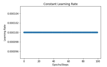
1. Constant Learning Rate 
In this section, we are training our neural network using a constant learning rate. We have set the number of epochs to 10, batch size to 256, and learning rate to 0.0001*. We have then initialized the model and its parameters. We have initialized the SGD optimizer with a constant learning rate. At last, we have called our training routine to train network. The function returns final updated parameters and validation accuracy.
We are maintaining a dictionary where we'll be storing the validation accuracy of all schedulers for comparison purposes later.
Later on, we have also plotted a chart showing the constant learning rate throughout the training process. We'll be plotting a chart like this for all our schedules to show how the learning rate is changing through the training process.
scheduler_val_accs = {}
seed = random.PRNGKey(0)
batch_size=256
epochs=10
learning_rate = jnp.array(1/1e4)

model = CNN()
weights = model.init(seed, X_train[:5])

optimizer = optax.sgd(learning_rate=learning_rate) ## Initialize SGD Optimizer
#constant_scheduler = optax.constant_schedule(0.0001)
#optimizer = optax.sgd(learning_rate=constant_scheduler)
optimizer_state = optimizer.init(weights)

final_weights, val_acc = TrainModelInBatches(X_train, Y_train, X_test, Y_test, epochs, weights, optimizer_state, batch_size=batch_size)
scheduler_val_accs["Constant Learning Rate"] = val_acc
import matplotlib.pyplot as plt

constant_scheduler = optax.constant_schedule(0.0001)

lrs = [constant_scheduler(i) for i in range(100)]

plt.scatter(range(100), lrs)
plt.title("Constant Learning Rate")
plt.ylabel("Learning Rate")
plt.xlabel("Epochs/Steps");
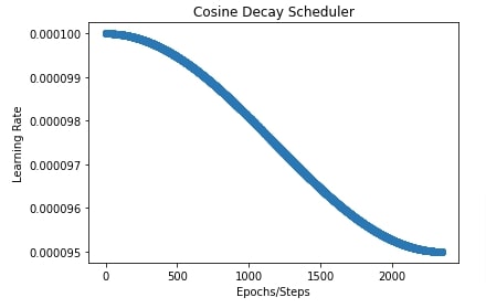
2. Cosine Decay Scheduler 
In this section, we are training our network with a cosine decay scheduler. We can create cosine decay scheduler using cosine_decay_schedule() function of optax. It accepts the initial learning rate and the total number of decay steps. It'll then decay learning rate in cosine curve fashion for those many steps. Here, one step is the execution of one batch of data. We can retrieve a total number of batches (steps) per epoch by dividing the number of train samples by batch size. Then, we can retrieve the total number of batches (steps) per training by multiplying the number of epochs by batches per epoch. This will constantly reduce the learning rate for all batches of training data.
The scheduler is a function that can take as input a step number and it'll return the learning rate to use for that step. Below is the formula used by the cosine decay scheduler to retrieve the learning rate for any step of training. We have tried to include the internal logic of the majority of schedulers for anyone who wants to know how they work internally. We have retrieved logic from optax documentation.
def scheduler(step_number):
        count = minimum(count, decay_steps)
        cosine_decay = 0.5 * (1 + cos(pi * step_number / decay_steps))
        decayed = (1 - alpha) * cosine_decay + alpha
        return  init_learning_rate * decayed
In order to use schedulers, we need to initialize them and provide them to SGD optimizer. It'll then reduce the learning rate using the above formula. All the schedulers can be used the same way through SGD.
After training the network with the scheduler, we have stored validation accuracy in our dictionary.
In the next cell, we have also plotted a chart to show how the learning rate will change over time during training using a cosine decay scheduler. This can help us better understand how it works.
seed = random.PRNGKey(0)
batch_size=256
epochs=10
learning_rate = jnp.array(1/1e4)

model = CNN()
weights = model.init(seed, X_train[:5])

total_steps = epochs*(X_train.shape[0]//batch_size) + epochs ## Total Batches
cosine_decay_scheduler = optax.cosine_decay_schedule(0.0001, decay_steps=total_steps, alpha=0.95)
optimizer = optax.sgd(learning_rate=cosine_decay_scheduler) ## Initialize SGD Optimizer
optimizer_state = optimizer.init(weights)

final_weights, val_acc = TrainModelInBatches(X_train, Y_train, X_test, Y_test, epochs, weights, optimizer_state, batch_size=batch_size)
scheduler_val_accs["Cosine Decay Scheduler"] = val_acc
import matplotlib.pyplot as plt

total_steps = epochs*(X_train.shape[0]//batch_size) + epochs
cosine_decay_scheduler = optax.cosine_decay_schedule(0.0001, decay_steps=total_steps, alpha=0.95)

lrs = [cosine_decay_scheduler(i) for i in range(total_steps)]

plt.scatter(range(total_steps), lrs)
plt.title("Cosine Decay Scheduler")
plt.ylabel("Learning Rate")
plt.xlabel("Epochs/Steps");
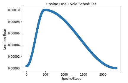
3. Cosine One Cycle Scheduler 
In this section, we are training our network using a cosine one-cycle scheduler. We can create cosine one cycle scheduler using cosine_onecycle_schedule() function available from optax. It has a list of the below parameters. Some have default values and are optional.
- transition_steps - Total number of steps over which learning rate changes.
- peak_value - The maximum value that the learning rate can attain.
- pct_start - The percentage of steps to keep increasing learning rate to peak_value. Default is 0.3.
- div_factor - It is used to determine initial learning rate. initial_learning_rate = peak_value / div_factor. Default is 25.0.
- final_div_factor - It is used to determine final learning rate at the end of training. final_learning_rate = initial_learning_rate / final_div_factor. Default value is 10000.0.
Below, scheduler logic is used to retrieve the learning rate of any step number during training.
def _cosine_interpolate(start: float, end: float, pct: float):
    return end + (start-end) / 2.0 * (jnp.cos(jnp.pi * pct) + 1)

def scheduler(step_number):
    init_learning_rate = peak_value / div_factor
    boundaries_and_scales = {int(pct_start * transition_steps): div_factor,
                             int(transition_steps): 1. / (div_factor * final_div_factor)}
    boundaries, scales = zip(*sorted(boundaries_and_scales.items()))
    bounds = np.stack((0,) + boundaries)
    values = np.cumprod(jnp.stack((init_learning_rate,) + scales))
    interval_sizes = (bounds[1:] - bounds[:-1])
    indicator = (bounds[:-1] <= step_number) & (step_number < bounds[1:])
    pct = (step_number - bounds[:-1]) / interval_sizes
    interp_vals = _cosine_interpolate(values[:-1], values[1:], pct)
    return indicator.dot(interp_vals) + (bounds[-1] <= step_number) * values[-1]
In our case, we have set peak value to 0.001, percentage start to 0.20 (20 %), division factor to 30, and final division factor to 100.
seed = random.PRNGKey(0)
batch_size=256
epochs=10
learning_rate = jnp.array(1/1e4)

model = CNN()
weights = model.init(seed, X_train[:5])

total_steps = epochs*(X_train.shape[0]//batch_size) + epochs
cosine_onecycle_scheduler = optax.cosine_onecycle_schedule(transition_steps=total_steps, peak_value=0.0001,
                                                           pct_start=0.20, div_factor=30., final_div_factor=100.)
optimizer = optax.sgd(learning_rate=cosine_onecycle_scheduler) ## Initialize SGD Optimizer
optimizer_state = optimizer.init(weights)

final_weights, val_acc = TrainModelInBatches(X_train, Y_train, X_test, Y_test, epochs, weights, optimizer_state, batch_size=batch_size)
scheduler_val_accs["Cosine One Cycle Scheduler"] = val_acc
import matplotlib.pyplot as plt

total_steps = epochs*(X_train.shape[0]//batch_size) + epochs
cosine_onecycle_scheduler = optax.cosine_onecycle_schedule(transition_steps=total_steps, peak_value=0.0001,
                                                           pct_start=0.20, div_factor=30., final_div_factor=100.)

lrs = [cosine_onecycle_scheduler(i) for i in range(total_steps)]

plt.scatter(range(total_steps), lrs)
plt.title("Cosine One Cycle Scheduler")
plt.ylabel("Learning Rate")
plt.xlabel("Epochs/Steps");
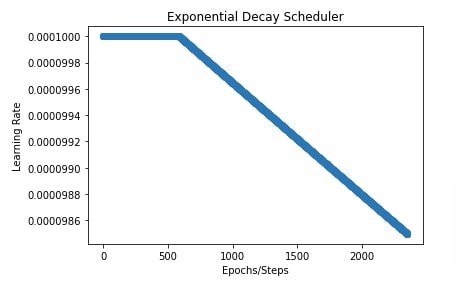
4. Exponential Decay 
In this section, we are training our network using an exponential decay scheduler to reduce the learning rate over time. We can create exponential decay scheduler using exponential_decay() method of optax library. The method takes the below parameters. Some of them have default values hence are optional.
- init_value - This is initial learning rate.
- transition_steps - Total number of training steps.
- decay_rate - The rate of decaying learning rate.
- transition_begin - Integer value specifying step number at which to begin decaying learning rate. The default value is 0 hence decaying starts at the beginning.
- staircase - It accepts boolean value which is set to True will decay value at discrete intervals. Default is False.
- end_value - It's the value at which the decaying of the learning rate stops. The learning rate won't decay below this value. Default is None.
def scheduler(step_number):
    decayed_value = init_learning_rate * decay_rate ^ (step_number / transition_steps)
    return decayed_value
Below, we have trained our network for 10 epochs using SGD with exponential decay. We are starting transition at 25% steps hence our learning rate will stay constant for the first 25% steps.
seed = random.PRNGKey(0)
batch_size=256
epochs=10
learning_rate = jnp.array(1/1e4)

model = CNN()
weights = model.init(seed, X_train[:5])

total_steps = epochs*(X_train.shape[0]//batch_size) + epochs
exponential_decay_scheduler = optax.exponential_decay(init_value=0.0001, transition_steps=total_steps,
                                                      decay_rate=0.98, transition_begin=int(total_steps*0.25),
                                                      staircase=False)
optimizer = optax.sgd(learning_rate=exponential_decay_scheduler) ## Initialize SGD Optimizer
optimizer_state = optimizer.init(weights)

final_weights, val_acc = TrainModelInBatches(X_train, Y_train, X_test, Y_test, epochs, weights, optimizer_state, batch_size=batch_size)
scheduler_val_accs["Exponential Decay"] = val_acc
import matplotlib.pyplot as plt

total_steps = epochs*(X_train.shape[0]//batch_size) + epochs
exponential_decay_scheduler = optax.exponential_decay(init_value=0.0001, transition_steps=total_steps,
                                                      decay_rate=0.98, transition_begin=int(total_steps*0.25),
                                                      staircase=False)

lrs = [exponential_decay_scheduler(i) for i in range(total_steps)]

plt.scatter(range(total_steps), lrs)
plt.title("Exponential Decay Scheduler")
plt.ylabel("Learning Rate")
plt.xlabel("Epochs/Steps");
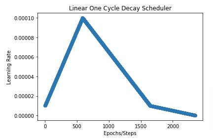
5. Linear One Cycle Scheduler 
In this section, we are training our network with a linear one-cycle scheduler with SGD. We can create linear one cycle scheduler using linear_onecycle_schedule() function of optax library. It has a list of the below parameters. Some of the parameters are optional and have default values.
- transition_steps - It accepts a number of steps for which to reduce the learning rate.
- peak_value - It accepts maximum value of learning rate.
- pct_start - It accepts float in the range [0,1] specifying for the percentage of steps the learning rate should keep increasing.
- pct_final - It accepts float in the range [0,1] specifying for how many percentages of steps the learning rate should increase and then decrease to an initial value.
- div_factor - It helps in determining initial value of learning rate. initial_learning_rate = peak_value / div_factor.
- final_div_factor - It helps in determining final learning rate. final_learning_rate = initial_learning_rate / final_div_factor.
Below, we have included code that is used internally by optax to determine the learning rate at each step.
def _linear_interpolate(start: float, end: float, pct: float):
    return (end-start) * pct + start

def scheduler(step_number):
    init_learning_rate = peak_value / div_factor
    boundaries_and_scales = {int(pct_start * transition_steps): div_factor,
                             int(transition_steps): 1. / (div_factor * final_div_factor)}
    boundaries, scales = zip(*sorted(boundaries_and_scales.items()))
    bounds = np.stack((0,) + boundaries)
    values = np.cumprod(jnp.stack((init_learning_rate,) + scales))
    interval_sizes = (bounds[1:] - bounds[:-1])
    indicator = (bounds[:-1] <= step_number) & (step_number < bounds[1:])
    pct = (step_number - bounds[:-1]) / interval_sizes
    interp_vals = _linear_interpolate(values[:-1], values[1:], pct)
    return indicator.dot(interp_vals) + (bounds[-1] <= step_number) * values[-1]
In our case, we have set peak value at 0.0001, percent start a 25%, percent final at 70%, division factor for initial learning rate at 10 (initial lr = 0.00001) and final division factor at 100 (final lr = 0.000001).
In the next cell after the below cell, we have also plotted a chart showing how the learning rate changes over time during the training process.
seed = random.PRNGKey(0)
batch_size=256
epochs=10
learning_rate = jnp.array(1/1e4)

model = CNN()
weights = model.init(seed, X_train[:5])

total_steps = epochs*(X_train.shape[0]//batch_size) + epochs
linear_onecycle_decay_scheduler = optax.linear_onecycle_schedule(transition_steps=total_steps, peak_value=0.0001,
                                                                 pct_start=0.25, pct_final=0.7, div_factor=10.,
                                                                 final_div_factor=100.)
optimizer = optax.sgd(learning_rate=linear_onecycle_decay_scheduler) ## Initialize SGD Optimizer
optimizer_state = optimizer.init(weights)

final_weights, val_acc = TrainModelInBatches(X_train, Y_train, X_test, Y_test, epochs, weights, optimizer_state, batch_size=batch_size)
scheduler_val_accs["Linear One Cycle Scheduler"] = val_acc
import matplotlib.pyplot as plt

total_steps = epochs*(X_train.shape[0]//batch_size) + epochs
linear_onecycle_decay_scheduler = optax.linear_onecycle_schedule(transition_steps=total_steps, peak_value=0.0001,
                                                                 pct_start=0.25, pct_final=0.7,
                                                                 div_factor=10., final_div_factor=100.)

lrs = [linear_onecycle_decay_scheduler(i) for i in range(total_steps)]

plt.scatter(range(total_steps), lrs)
plt.title("Linear One Cycle Decay Scheduler")
plt.ylabel("Learning Rate")
plt.xlabel("Epochs/Steps");
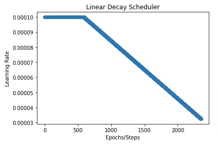
6. Linear Scheduler 
In this section, we have trained our CNN using SGD with the linear scheduler. We can create linear scheduler using linear_schedule() function. It accepts a list of the below parameters.
- init_value - Initial learning rate.
- end_value - Final learning rate at the end of training.
- transition_steps - Total number of steps.
- transition_begin - Step number from which to start reducing learning rate.
def scheduler(step_number):
    count = np.clip(step_number - transition_begin, 0, transition_steps)
    frac = 1 - step_number / transition_steps
    return (init_value - end_value) * frac + end_value
  return schedule
In our case below, we have set the initial learning rate to 0.0001, the final learning rate to 0.00001 and the transition begin after the first 25% steps.
In the next cell, we have plotted a chart showing how the learning rate will change over time during training.
seed = random.PRNGKey(0)
batch_size=256
epochs=10
learning_rate = jnp.array(1/1e4)

model = CNN()
weights = model.init(seed, X_train[:5])

total_steps = epochs*(X_train.shape[0]//batch_size) + epochs
linear_decay_scheduler = optax.linear_schedule(init_value=0.0001, end_value=0.00001,
                                               transition_steps=total_steps,
                                               transition_begin=int(total_steps*0.25))
optimizer = optax.sgd(learning_rate=linear_decay_scheduler) ## Initialize SGD Optimizer
optimizer_state = optimizer.init(weights)

final_weights, val_acc = TrainModelInBatches(X_train, Y_train, X_test, Y_test, epochs, weights, optimizer_state, batch_size=batch_size)
scheduler_val_accs["Linear Scheduler"] = val_acc
import matplotlib.pyplot as plt

total_steps = epochs*(X_train.shape[0]//batch_size) + epochs
linear_decay_scheduler = optax.linear_schedule(init_value=0.0001, end_value=0.00001,
                                               transition_steps=total_steps,
                                               transition_begin=int(total_steps*0.25))

lrs = [linear_decay_scheduler(i) for i in range(total_steps)]

plt.scatter(range(total_steps), lrs)
plt.title("Linear Decay Scheduler")
plt.ylabel("Learning Rate")
plt.xlabel("Epochs/Steps");
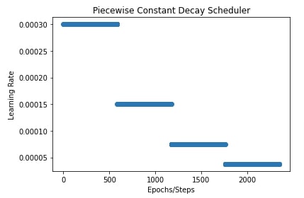
7. Piecewise Constant Scheduler 
In this section, we have trained our CNN using SGD with the piecewise constant scheduler. We can create piecewise constant scheduler using piecewise_constant_schedule() function. Below is a list of parameters of the function.
- init_value - Initial learning rate.
- boundaries_and_scales - It is a mapping from step number to scaling factor. It'll take step number from this mapping and after those many steps have passed, it'll scale the current learning rate by the value of step number in mapping.
Below, we have included code that optax uses internally to reduce the learning rate over time.
def scheduler(step_number):
    v = init_value
    if boundaries_and_scales is not None:
    for threshold, scale in sorted(boundaries_and_scales.items()):
        indicator = np.maximum(0., np.sign(step_number - count))
        v = v * indicator + (1 - indicator) * scale * v
    return v
In our case, we have set the initial learning rate to 0.0003. Then, mapping has 3 entries. The 25% steps, 50% steps, and 75% steps, all of which have a factor of 0.5. This will inform the scheduler that after 25% steps are passed, scale learning rate by 0.5, scale it by another 0.5 amount after 50% steps has passed, and finally after 75% has passed, scale it again by 0.5.
In the next cell, we have also plotted a chart showing how the learning rate will change that can make things clear to understand.
seed = random.PRNGKey(0)
batch_size=256
epochs=10
learning_rate = jnp.array(1/1e4)

model = CNN()
weights = model.init(seed, X_train[:5])

total_steps = epochs*(X_train.shape[0]//batch_size) + epochs
piecewise_constant_decay_scheduler = optax.piecewise_constant_schedule(init_value=0.0003,
                                                               boundaries_and_scales={int(total_steps*0.25):0.5,
                                                                                      int(total_steps*0.5):0.5,
                                                                                      int(total_steps*0.75):0.5})
optimizer = optax.sgd(learning_rate=piecewise_constant_decay_scheduler) ## Initialize SGD Optimizer
optimizer_state = optimizer.init(weights)

final_weights, val_acc = TrainModelInBatches(X_train, Y_train, X_test, Y_test, epochs, weights, optimizer_state, batch_size=batch_size)
scheduler_val_accs["Piecewise Constant Scheduler"] = val_acc
import matplotlib.pyplot as plt

total_steps = epochs*(X_train.shape[0]//batch_size) + epochs
piecewise_constant_decay_scheduler = optax.piecewise_constant_schedule(init_value=0.0003, boundaries_and_scales={int(total_steps*0.25):0.5, int(total_steps*0.5):0.5, int(total_steps*0.75):0.5})

lrs = [piecewise_constant_decay_scheduler(i) for i in range(total_steps)]

plt.scatter(range(total_steps), lrs)
plt.title("Piecewise Constant Decay Scheduler")
plt.ylabel("Learning Rate")
plt.xlabel("Epochs/Steps");
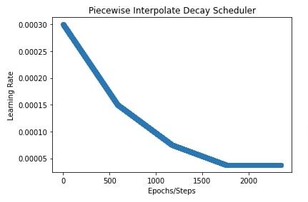
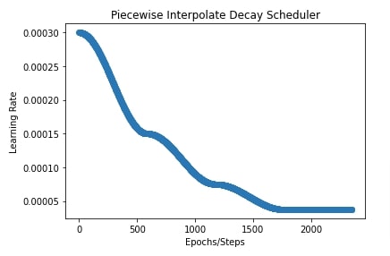
8. Piecewise Interpolate Scheduler 
In this section, we have trained our CNN using SGD with a piece-wise interpolate scheduler. We can create piecewise interpolate scheduler using piecewise_interpolate_schedule() function. It has the below-mentioned parameters.
- interpolate_type - It accepts one of the below string values.
- 'linear'
- 'cosine'
- init_value - Initial learning rate
- boundaries_and_scales - This is a mapping which works same as we explained in previous piece wise constant scheduler.
Below, we have included logic on how the calculation of learning rate is done during training.
def _linear_interpolate(start: float, end: float, pct: float):
    return (end-start) * pct + start

def _cosine_interpolate(start: float, end: float, pct: float):
    return end + (start-end) / 2.0 * (jnp.cos(jnp.pi * pct) + 1)

def scheduler(step_number):
    if interpolate_type == 'linear':
        interpolate_fn = _linear_interpolate
    elif interpolate_type == 'cosine':
        interpolate_fn = _cosine_interpolate
    else:
        raise ValueError('`interpolate_type` must be either \'cos\' or \'linear\'')

    if boundaries_and_scales:
        boundaries, scales = zip(*sorted(boundaries_and_scales.items()))
    else:
        boundaries, scales = (), ()
    bounds = np.stack((0,) + boundaries)
    values = np.cumprod(np.stack((init_value,) + scales))
    interval_sizes = (bounds[1:] - bounds[:-1])
    indicator = (bounds[:-1] <= count) & (count < bounds[1:])
    pct = (count - bounds[:-1]) / interval_sizes
    interp_vals = interpolate_fn(values[:-1], values[1:], pct)
    return indicator.dot(interp_vals) + (bounds[-1] <= count) * values[-1]
Below, we have initialized our scheduler with interpolate type as 'linear' and initial learning rate of 0.0003. The boundaries and scales parameter is the same as in our previous example.
In the next cell, we have also plotted learning rate change over time to give a better idea of how the scheduler works.
seed = random.PRNGKey(0)
batch_size=256
epochs=10
learning_rate = jnp.array(1/1e4)

model = CNN()
weights = model.init(seed, X_train[:5])

total_steps = epochs*(X_train.shape[0]//batch_size) + epochs
piecewise_interpolate_decay_scheduler = optax.piecewise_interpolate_schedule(interpolate_type="linear",
                                                                             init_value=0.0003,
                                                                boundaries_and_scales={int(total_steps*0.25):0.5,
                                                                                       int(total_steps*0.5):0.5,
                                                                                       int(total_steps*0.75):0.5})
optimizer = optax.sgd(learning_rate=piecewise_interpolate_decay_scheduler) ## Initialize SGD Optimizer
optimizer_state = optimizer.init(weights)

final_weights, val_acc = TrainModelInBatches(X_train, Y_train, X_test, Y_test, epochs, weights, optimizer_state, batch_size=batch_size)
scheduler_val_accs["Piecewise Interpolate Scheduler V1"] = val_acc
import matplotlib.pyplot as plt

total_steps = epochs*(X_train.shape[0]//batch_size) + epochs
piecewise_interpolate_decay_scheduler = optax.piecewise_interpolate_schedule(interpolate_type="linear",
                                                                             init_value=0.0003,
                                                                boundaries_and_scales={int(total_steps*0.25):0.5,
                                                                                       int(total_steps*0.5):0.5,
                                                                                       int(total_steps*0.75):0.5})

lrs = [piecewise_interpolate_decay_scheduler(i) for i in range(total_steps)]

plt.scatter(range(total_steps), lrs)
plt.title("Piecewise Interpolate Decay Scheduler")
plt.ylabel("Learning Rate")
plt.xlabel("Epochs/Steps");
In the below cell, we are training our CNN again using a piece-wise interpolate scheduler. The scheduler has the same setting as the above example with only a change in interpolate type which is changed to 'cosine'.
In the next cell, we have also plotted a chart showing how the learning rate changes using this scheduler during training.
seed = random.PRNGKey(0)
batch_size=256
epochs=10
learning_rate = jnp.array(1/1e4)

model = CNN()
weights = model.init(seed, X_train[:5])

total_steps = epochs*(X_train.shape[0]//batch_size) + epochs
piecewise_interpolate_decay_scheduler = optax.piecewise_interpolate_schedule(interpolate_type="cosine",
                                                                             init_value=0.0003,
                                                                boundaries_and_scales={int(total_steps*0.25):0.5,
                                                                                       int(total_steps*0.5):0.5,
                                                                                       int(total_steps*0.75):0.5})
optimizer = optax.sgd(learning_rate=piecewise_interpolate_decay_scheduler) ## Initialize SGD Optimizer
optimizer_state = optimizer.init(weights)

final_weights, val_acc = TrainModelInBatches(X_train, Y_train, X_test, Y_test, epochs, weights, optimizer_state, batch_size=batch_size)
scheduler_val_accs["Piecewise Interpolate Scheduler V2"] = val_acc
import matplotlib.pyplot as plt

total_steps = epochs*(X_train.shape[0]//batch_size) + epochs
piecewise_interpolate_decay_scheduler = optax.piecewise_interpolate_schedule(interpolate_type="cosine",
                                                                             init_value=0.0003,
                                                                boundaries_and_scales={int(total_steps*0.25):0.5,
                                                                                       int(total_steps*0.5):0.5,
                                                                                       int(total_steps*0.75):0.5})

lrs = [piecewise_interpolate_decay_scheduler(i) for i in range(total_steps)]

plt.scatter(range(total_steps), lrs)
plt.title("Piecewise Interpolate Decay Scheduler")
plt.ylabel("Learning Rate")
plt.xlabel("Epochs/Steps");
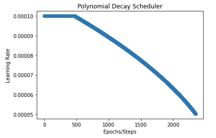
9. Polynomial Scheduler 
In this section, we have trained our CNN using SGD with the polynomial scheduler. We can create polynomial scheduler using polynomial_schedule() function. Below are important parameters of the function.
- init_value - Initial learning rate
- end_value - Final learning rate
- power - Power of polynomial equation used to transfer learning rate from initial value to final.
- transition_steps - Number of steps for which to reduce learning rate.
- transition_begin - Number of steps after which start learning rate annealing.
The below formula is used by optax to calculate the learning rate at any step of training.
def scheduler(step_number):
    count = np.clip(step_number - transition_begin, 0, transition_steps)
    frac = 1 - step_number / transition_steps
    return (init_value - end_value) * (frac**power) + end_value
In our case, we have set the initial learning rate to 0.0001, the final learning rate to 0.00001, power to 0.5, and transition begin to 20% steps.
In the next cell below after training, we have also plotted a chart showing how the learning rate changes during training.
seed = random.PRNGKey(0)
batch_size=256
epochs=10
learning_rate = jnp.array(1/1e4)

model = CNN()
weights = model.init(seed, X_train[:5])

total_steps = epochs*(X_train.shape[0]//batch_size) + epochs
polynomial_decay_scheduler = optax.polynomial_schedule(init_value=0.0001, end_value=0.00001,
                                                       power=0.5, transition_steps=total_steps,
                                                       transition_begin=int(total_steps*0.20))
optimizer = optax.sgd(learning_rate=piecewise_interpolate_decay_scheduler) ## Initialize SGD Optimizer
optimizer_state = optimizer.init(weights)

final_weights, val_acc = TrainModelInBatches(X_train, Y_train, X_test, Y_test, epochs, weights, optimizer_state, batch_size=batch_size)
scheduler_val_accs["Polynomial Scheduler"] = val_acc
import matplotlib.pyplot as plt

total_steps = epochs*(X_train.shape[0]//batch_size) + epochs
polynomial_decay_scheduler = optax.polynomial_schedule(init_value=0.0001, end_value=0.00001,
                                                       power=0.5, transition_steps=total_steps,
                                                       transition_begin=int(total_steps*0.20))

lrs = [polynomial_decay_scheduler(i) for i in range(total_steps)]

plt.scatter(range(total_steps), lrs)
plt.title("Polynomial Decay Scheduler")
plt.ylabel("Learning Rate")
plt.xlabel("Epochs/Steps");
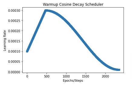
10. Warmup Cosine Decay Scheduler 
In this section, we have trained our CNN using SGD with a warmup cosine decay scheduler. We can create warmup cosine decay scheduler using warmup_cosine_decay_schedule() function. It takes the below-mentioned parameters.
- init_value - Initial learning rate.
- peak_value - Peak/Maximum learning rate.
- end_value - End learning rate.
- warmup_steps - Number of steps to reach from initial learning rate to peak learning rate linearly.
- decay_steps - Total number of steps for which learning rate annealing happens.
This scheduler first applies linear scheduler (Section 6 of this tutorial) to reach from initial learning rate to peak learning rate and then applies cosine decay scheduler (Section 2) to take learning rate from peak to final/end value.
In our case, we have set the initial learning rate to 0.0001, peak value to 0.0003, warmup steps to 20% of steps, and end value to 0.00001.
In the next cell after the training cell, we have plotted a chart showing how the learning rate changes during training.
seed = random.PRNGKey(0)
batch_size=256
epochs=10
learning_rate = jnp.array(1/1e4)

model = CNN()
weights = model.init(seed, X_train[:5])

total_steps = epochs*(X_train.shape[0]//batch_size) + epochs
warmup_cosine_decay_scheduler = optax.warmup_cosine_decay_schedule(init_value=0.0001, peak_value=0.0003,
                                                                   warmup_steps=int(total_steps*0.2),
                                                                   decay_steps=total_steps, end_value=0.00001)
optimizer = optax.sgd(learning_rate=warmup_cosine_decay_scheduler) ## Initialize SGD Optimizer
optimizer_state = optimizer.init(weights)

final_weights, val_acc = TrainModelInBatches(X_train, Y_train, X_test, Y_test, epochs, weights, optimizer_state, batch_size=batch_size)
scheduler_val_accs["Warmup Cosine Decay Scheduler"] = val_acc
import matplotlib.pyplot as plt

total_steps = epochs*(X_train.shape[0]//batch_size) + epochs
warmup_cosine_decay_scheduler = optax.warmup_cosine_decay_schedule(init_value=0.0001, peak_value=0.0003,
                                                                   warmup_steps=int(total_steps*0.2),
                                                                   decay_steps=total_steps, end_value=0.00001)

lrs = [warmup_cosine_decay_scheduler(i) for i in range(total_steps)]

plt.scatter(range(total_steps), lrs)
plt.title("Warmup Cosine Decay Scheduler")
plt.ylabel("Learning Rate")
plt.xlabel("Epochs/Steps");
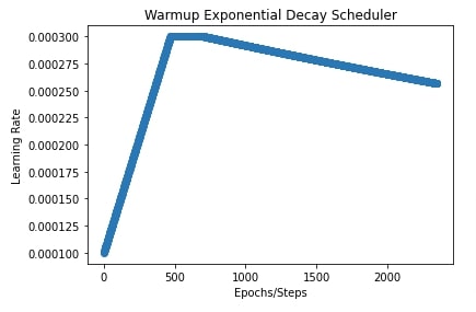
11. Warmup Exponential Decay Scheduler 
In this section, we have trained our CNN using SGD with a warmup exponential decay scheduler. We can create warmup exponential decay scheduler using warmup_exponential_decay_schedule() function. It takes the below-mentioned parameters.
- init_value - Initial learning rate.
- peak_value - Peak/maximum learning rate.
- end_value - Final/end learning rate.
- warmup_steps - Number of steps to reach from initial learning rate to peak learning rate linearly.
- transition_steps - Total number of steps for which learning rate annealing happens.
- decay_rate - Float value specifying exponential decay rate.
- transition_begin - Steps after which to begin annealing learning rate.
This scheduler first applies linear scheduler (Section 6 of this tutorial) to reach from initial learning rate to peak learning rate and then applies exponential decay scheduler (Section 4) to take learning rate from peak to final/end value.
In our case, the initial learning rate is 0.0001, the peak value is 0.0003, warmup steps are initial 20% steps, the decay rate is 0.8, the transition begins at 10% steps (after the first 20% steps of warmup) and end value of learning rate is 0.00001.
We have also plotted the learning rate to show how it changes during training.
seed = random.PRNGKey(0)
batch_size=256
epochs=10
learning_rate = jnp.array(1/1e4)

model = CNN()
weights = model.init(seed, X_train[:5])

total_steps = epochs*(X_train.shape[0]//batch_size) + epochs
warmup_exponential_decay_scheduler = optax.warmup_exponential_decay_schedule(init_value=0.0001, peak_value=0.0003,
                                                                             warmup_steps=int(total_steps*0.2),
                                                                             transition_steps=total_steps,
                                                                             decay_rate=0.8,
                                                                             transition_begin=int(total_steps*0.1),
                                                                             end_value=0.00001)

optimizer = optax.sgd(learning_rate=warmup_exponential_decay_scheduler) ## Initialize SGD Optimizer
optimizer_state = optimizer.init(weights)

final_weights, val_acc = TrainModelInBatches(X_train, Y_train, X_test, Y_test, epochs, weights, optimizer_state, batch_size=batch_size)
scheduler_val_accs["Warmup Exponential Decay Scheduler"] = val_acc
import matplotlib.pyplot as plt

total_steps = epochs*(X_train.shape[0]//batch_size) + epochs
warmup_exponential_decay_scheduler = optax.warmup_exponential_decay_schedule(init_value=0.0001, peak_value=0.0003,
                                                                             warmup_steps=int(total_steps*0.2),
                                                                             transition_steps=total_steps,
                                                                             decay_rate=0.8,
                                                                             transition_begin=int(total_steps*0.1),
                                                                             end_value=0.00001)

lrs = [warmup_exponential_decay_scheduler(i) for i in range(total_steps)]

plt.scatter(range(total_steps), lrs)
plt.title("Warmup Exponential Decay Scheduler")
plt.ylabel("Learning Rate")
plt.xlabel("Epochs/Steps");
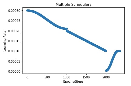
12. Combining Multiple Schedulers 
Optax also let us combine multiple schedulers if one of them is not sufficient for our case. It provides a method named join_schedules() that lets us combine multiple schedulers. We need to provide a list of schedulers and boundaries of steps to which to apply those schedulers.
In our case below, we have created three schedulers.
- cosine decay scheduler.
- linear scheduler.
- cosine one cycle scheduler.
We have set boundaries to [1000,2000]. This will apply a cosine decay scheduler to the first 1000 steps, a linear scheduler to steps from 1000 to 2000, and a cosine one cycle scheduler to the remaining steps after 2000.
We have also plotted how the learning rate will change during training with these combined schedulers.
seed = random.PRNGKey(0)
batch_size=256
epochs=10
learning_rate = jnp.array(1/1e4)

model = CNN()
weights = model.init(seed, X_train[:5])

total_steps = epochs*(X_train.shape[0]//batch_size) + epochs
cosine_decay_scheduler = optax.cosine_decay_schedule(0.0003, decay_steps=1000, alpha=0.7)
linear_decay_scheduler = optax.linear_schedule(init_value=0.0002, end_value=0.0001,
                                               transition_steps=1000)
cosine_onecycle_scheduler = optax.cosine_onecycle_schedule(transition_steps=1000, peak_value=0.0001,
                                                           div_factor=30., final_div_factor=1000.)

multiple_schedulers = optax.join_schedules([cosine_decay_scheduler, linear_decay_scheduler,
                                            cosine_onecycle_scheduler], boundaries=[1000, 2000])
optimizer = optax.sgd(learning_rate=multiple_schedulers) ## Initialize SGD Optimizer
optimizer_state = optimizer.init(weights)

final_weights, val_acc = TrainModelInBatches(X_train, Y_train, X_test, Y_test, epochs, weights, optimizer_state, batch_size=batch_size)
scheduler_val_accs["Combining Multiple Scheduler"] = val_acc
import matplotlib.pyplot as plt

total_steps = epochs*(X_train.shape[0]//batch_size) + epochs
cosine_decay_scheduler = optax.cosine_decay_schedule(0.0003, decay_steps=1000, alpha=0.7)
linear_decay_scheduler = optax.linear_schedule(init_value=0.0002, end_value=0.0001,
                                               transition_steps=1000)
cosine_onecycle_scheduler = optax.cosine_onecycle_schedule(transition_steps=1000, peak_value=0.0001,
                                                           div_factor=30., final_div_factor=1000.)

multiple_schedulers = optax.join_schedules([cosine_decay_scheduler, linear_decay_scheduler,
                                            cosine_onecycle_scheduler], boundaries=[1000, 2000])

lrs = [multiple_schedulers(i) for i in range(total_steps)]

plt.scatter(range(total_steps), lrs)
plt.title("Multiple Schedulers")
plt.ylabel("Learning Rate")
plt.xlabel("Epochs/Steps");
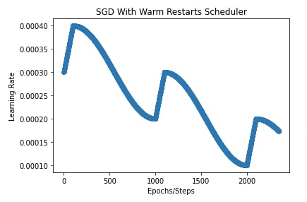
13. SGD With Warm Restarts 
In this section, we have trained our CNN using SGD with a warm restarts scheduler. We can initialize SGD with warm restarts scheduler using sgdr_schedule() function. It takes a list of dictionaries where each dictionary specifies parameters of the warmup cosine decay scheduler. It'll execute all warmup cosine decay schedulers one by one for a specified number of steps in configuration.
In our case, we have provided a list of three dictionaries to sgdr_schedule() function. Each specifies a different warmup cosine decay scheduler. The first entry asks to start learning rate from 0.0003 to the peak value of 0.0004 and then end at 0.0002. It'll run for the first 1000 steps. It'll take it 100 steps to each from 0.0003 to 0.0004. The same logic will be followed for the next 1000 steps using the second dictionary. Here, we'll take the learning rate from 0.0002 to 0.0003 and then drop it to 0.0001. For the last 1000 steps, we'll take the learning rate from 0.0001 to 0.0002 and then drop it to 0.00005.
We have also plotted how the learning rate will change during training using this scheduler.
seed = random.PRNGKey(0)
batch_size=256
epochs=10
learning_rate = jnp.array(1/1e4)

model = CNN()
weights = model.init(seed, X_train[:5])

total_steps = epochs*(X_train.shape[0]//batch_size) + epochs
sgd_with_warm_restarts_decay_scheduler = optax.sgdr_schedule(
    [{"init_value":0.0003, "peak_value":0.0004, "decay_steps":1000, "warmup_steps":100, "end_value":0.0002},
     {"init_value":0.0002, "peak_value":0.0003, "decay_steps":1000, "warmup_steps":100, "end_value":0.0001},
     {"init_value":0.0001, "peak_value":0.0002, "decay_steps":1000, "warmup_steps":100, "end_value":0.00005},
    ]
)
optimizer = optax.sgd(learning_rate=sgd_with_warm_restarts_decay_scheduler) ## Initialize SGD Optimizer
optimizer_state = optimizer.init(weights)

final_weights, val_acc = TrainModelInBatches(X_train, Y_train, X_test, Y_test, epochs, weights, optimizer_state, batch_size=batch_size)
scheduler_val_accs["SGD With Warm Restarts"] = val_acc
import matplotlib.pyplot as plt

total_steps = epochs*(X_train.shape[0]//batch_size) + epochs
sgd_with_warm_restarts_decay_scheduler = optax.sgdr_schedule(
    [{"init_value":0.0003, "peak_value":0.0004, "decay_steps":1000, "warmup_steps":100, "end_value":0.0002},
     {"init_value":0.0002, "peak_value":0.0003, "decay_steps":1000, "warmup_steps":100, "end_value":0.0001},
     {"init_value":0.0001, "peak_value":0.0002, "decay_steps":1000, "warmup_steps":100, "end_value":0.00005},
    ]
)

lrs = [sgd_with_warm_restarts_decay_scheduler(i) for i in range(total_steps)]

plt.scatter(range(total_steps), lrs)
plt.title("SGD With Warm Restarts Scheduler")
plt.ylabel("Learning Rate")
plt.xlabel("Epochs/Steps");
Final Test/Valid Set Accuracy Comparison of Various Schedulers 
In this section, we have simply created a dataframe from validation accuracy that we had stored in the dictionary for all schedulers for comparison purposes.
import pandas as pd

pd.DataFrame(scheduler_val_accs, index=["Valid Accuracy"]).T
This ends our small tutorial explaining how we can use learning rate schedulers available from optax library for our Flax/JAX networks. We can easily create a custom scheduler as well for Flax/JAX networks as all of the schedulers are basically function that takes as input step number and returns learning rate for that step. Please feel free to let us know your views in the comments section.
References
 Sunny Solanki
Sunny Solanki
Intro: Software Developer | Youtuber | Bonsai Enthusiast
About: Sunny Solanki holds a bachelor's degree in Information Technology (2006-2010) from L.D. College of Engineering. Post completion of his graduation, he has 8.5+ years of experience (2011-2019) in the IT Industry (TCS). His IT experience involves working on Python & Java Projects with US/Canada banking clients. Since 2020, he’s primarily concentrating on growing CoderzColumn.
His main areas of interest are AI, Machine Learning, Data Visualization, and Concurrent Programming. He has good hands-on with Python and its ecosystem libraries.
Apart from his tech life, he prefers reading biographies and autobiographies. And yes, he spends his leisure time taking care of his plants and a few pre-Bonsai trees.
Contact: sunny.2309@yahoo.in


![YouTube Subscribe]() Comfortable Learning through Video Tutorials?
Comfortable Learning through Video Tutorials?
If you are more comfortable learning through video tutorials then we would recommend that you subscribe to our YouTube channel.
![Need Help]() Stuck Somewhere? Need Help with Coding? Have Doubts About the Topic/Code?
Stuck Somewhere? Need Help with Coding? Have Doubts About the Topic/Code?
 Stuck Somewhere? Need Help with Coding? Have Doubts About the Topic/Code?
When going through coding examples, it's quite common to have doubts and errors.
If you have doubts about some code examples or are stuck somewhere when trying our code, send us an email at coderzcolumn07@gmail.com. We'll help you or point you in the direction where you can find a solution to your problem.
You can even send us a mail if you are trying something new and need guidance regarding coding. We'll try to respond as soon as possible.
![Share Views]() Want to Share Your Views? Have Any Suggestions?
Want to Share Your Views? Have Any Suggestions?
 Want to Share Your Views? Have Any Suggestions?
If you want to
- provide some suggestions on topic
- share your views
- include some details in tutorial
- suggest some new topics on which we should create tutorials/blogs
 optax, learning-rate-schedules