Geoviews - Scatter & Bubble Maps
Geoviews is a Python library that lets us plot our geospatial data on Maps. It let us create maps like choropleth maps, scatter maps, bubble maps, etc. Geoviews is built on the top of the library named holoviews. It let us declare metadata about our map and then uses this metadata to create maps. It does not create maps on its own, instead, it uses one of the bokeh or matplotlib as a backend to create maps. We can set whichever backend we want to use using geoviews and then it'll create maps using that backend. The maps created using bokeh will be interactive maps whereas the ones create with matplotlib will be static maps. As a part of this tutorial, we'll explain with simple examples how we can create scatter and bubble maps using geoviews. We'll be using datasets available from geopandas and a few from the internet to create maps in our tutorial. We have already covered the tutorial on creating choropleth maps using geoviews. Please check the below link if you want to create choropleth maps.
If you are interested in learning about holoviews on which geoviews is based then please check our tutorial on it. It'll help you with this tutorial as well.
We'll now start our tutorial by importing geoviews and printing the version of it.
import geoviews

print("Geoviews Version : {}".format(geoviews.__version__))
We'll first load a few datasets, to begin with. We'll be merging a few of these datasets as per our need to create maps.
The first dataset that we have loaded below is the world geometry dataset available from geopandas. It's an object of type GeoDataFrame which has information about the geometry of each country of the world. It has information about polygon/multi-polygon objects for each country of the world which will be used to plot countries on the map. We'll be using this dataset to create a world map and then plot points/bubbles on it.
If you want to learn about geopandas then please feel free to check our tutorial on it.
import geopandas as gpd

print("Geopandas Version : {}".format(gpd.__version__))

print("Available Datasets : {}".format(gpd.datasets.available))

world = gpd.read_file(gpd.datasets.get_path("naturalearth_lowres"))

world.head()
Below we have loaded another dataset that has information about the happiness score of each country of the world. Apart from the happiness score, it has information like GDP per capita, life expectancy, social support, freedom, generosity, and perception of corruption. This dataset does not have geometry information hence it'll be loaded as simple pandas dataframe. This dataframe will be merged with other geo data frames to add information of this dataframe to them. The dataset can be downloaded from the below link.
import pandas as pd

happiness = pd.read_csv("datasets/world_happiness_2019.csv")

happiness.head()
The third dataset that we have loaded has information about stores of Starbucks worldwide. It has Longitude and Latitude of each store. Apart from this, it has information like store name, address, city, state, country, postcode, phone number, etc. We have loaded this dataset as simple pandas dataframe. The dataset can be downloaded from the below link.
starbucks = pd.read_csv("datasets/starbucks_store_locations.csv")

starbucks.head()
Scatter Maps
In this section, we'll explain how we can create scatter maps using geoviews. We have first set backend as bokeh using extension() method of geoviews. We can use the same method if we want to use matplotlib as a backend for our maps.
geoviews.extension("bokeh")

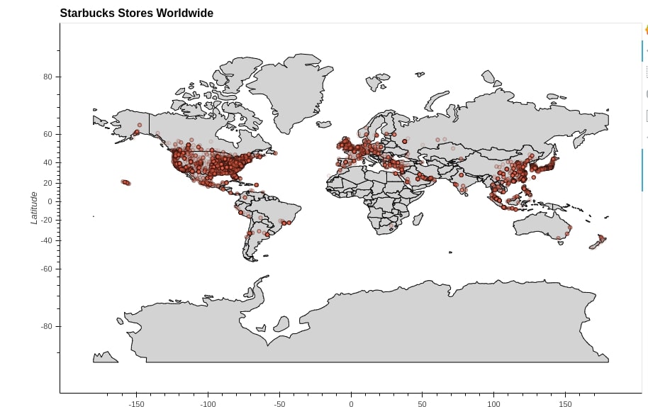
Starbucks Store Locations Worldwide Scatter Map
Our first scatter map shows locations of Starbucks stores on the world map. In order to create a world map, we have used Polygons() method. We have given it the world geo dataframe that we had loaded earlier using geopandas. This will create an empty world map. We have explained in detail how Polygons() method work in our tutorial on choropleth maps using geoviews.
In order to plot points on the map showing locations of Starbucks stores, we need to use Points() method of geoviews. Below we have given a definition of the method for explanation purposes.
- Points(data,kdims=[],vdims=[],**kwargs) - This method accepts normal pandas dataframe or geo dataframe along with other parameters and creates points on locations based on parameters settings.
- The data parameter can take normal pandas dataframe which has latitude and longitude columns or geopandas GeoDataFrame which has Point objects (representing location on map) in geometry column.
- The kdims parameter accepts a list of two strings where the first string is column name from the dataframe where Longitude information is present and the second string is where Latitude information is present. The points will be drawn at those locations. If we have given GeoDataFrame where geometry column has shapely Point objects in them then we can ignore this parameter as that column's data will be used to plot points on a map.
- The vdims parameter accepts a list of strings as input which are column names in the dataframe. The first string column name will be used to decide the sizes of points on a map and all other columns will be used to show data in a tooltip when the mouse hovers over the point.
After creating a world map using Polygons() method, we have created the plot of points using Points() method by giving it the Starbucks dataset that we loaded earlier. We have asked it to use Longitude and Latitude columns for kdims parameter and Store Name and City columns for vdims parameter. As Store Name is a column with string values, all points will be of the same size.
We have then merged the world map created using Polygons() with points plot created using Points() using simple multiplication. This is the standard way of combining more than one plot in library holoviews on top of which geoviews is built. We recommend that you go through our tutorial on holoviews to understand this if you don't have a background on this.
Apart from creating a map, we have set modified various map attributes like height, width, title, points color, points size, opacity, etc. We have done that in two ways. Holoviews lets us modify various attributes of maps in two ways.
- %%opts Cell Magic Command - This is cell magic command in jupyter notebooks which is available for charts created through holoviews. It accepts the first argument which is the name of the object (Polygons or Points in our case). Then it let us specify chart parameters to modify in two ways.
- The parameters mentioned in [] let us modify overall chart dimensions like height, width, title, axes, labels, ticks, tools, axes limits, etc.
- The parameters mentioned in () let us modify the look of components inside of map, like colormap of regions, opacity, hover color, etc.
- If you want to learn about magic commands in a jupyter notebook then please feel free to check our small tutorial explaining them with simple examples. List of Useful Magic Commands in Jupyter Notebook
- opts() Method - This method can be called on an instance of Points by giving a list of parameters and their values one after another. There is no distinction like %%opts cell magic command here.
In our example, we have specified Polygons options using cell magic command and Points options using opts() method. In our upcoming examples, we'll give Points options also using cell magic commands. It's a choice of the developer which method he/she wants to use.
%%opts Polygons [height=600 width=900 tools=["hover", ] title="Starbucks Stores Worldwide"] (color="lightgrey")

world_map = geoviews.Polygons(world)

points_on_map = geoviews.Points(starbucks,
                                kdims=["Longitude", "Latitude"],
                                vdims=["Store Name", "City"]).opts(color="tomato",
                                                           size=5,
                                                           alpha=0.1,
                                                           line_color="black",
                                                           hover_color="lime",
                                                           tools=["hover", ]
                                                        )

world_map * points_on_map
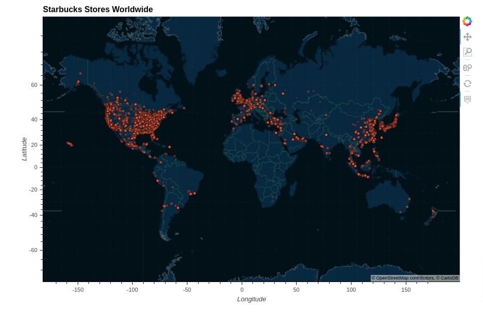
Starbucks Stores Worldwide Scatter Map (CartoMidnight Tile)
In this example, we have again created Starbucks stores scatter map but this time we have created a background map using tile service provided by bokeh. There are various geo tile providers which present different types of information on the map and we can add that information to our map by just adding that tile to our map. The tile can have information like world countries’ names, a terrain view, midnight view, topographic view, ocean view of the world.
Below we have created points using Points() method like our previous example. We have then merged this point object with CartoMidnight tile using star operation. There are various tiles available through geoviews.tile_sources module. We can retrieve a list of all possible available tiles using geoviews.tile_sources.tile_sources command.
Please make a NOTE that we have set a few options of Points using cell magic command this time.
%%opts Points [height=600 width=900 title="Starbucks Stores Worldwide"]

points_on_map = geoviews.Points(
                                starbucks,
                                kdims=["Longitude", "Latitude"],
                                vdims=["Store Name", "City"],
                        ).opts(color="tomato",
                               size=5,
                               alpha=0.1,
                               line_color="black",
                               hover_color="lime",
                               tools=["hover", ]
                        )


points_on_map * geoviews.tile_sources.CartoMidnight()
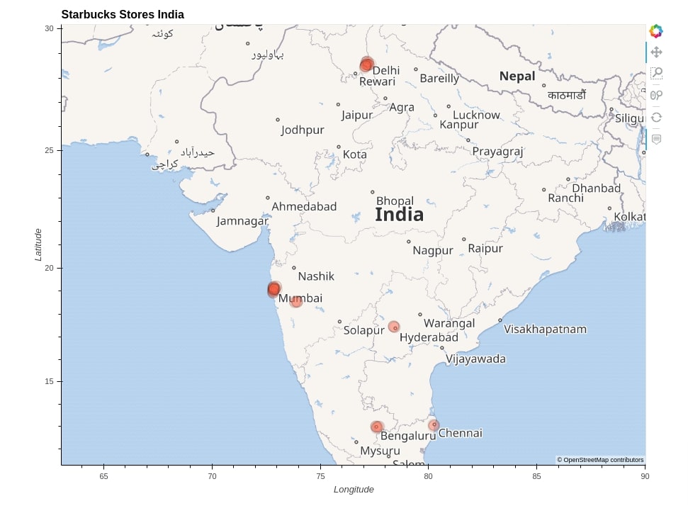
Starbucks Store Locations Across India
In this example, we have created a scatter map showing Starbucks store locations across India. We have created points on a map using Points() method by giving it a filtered Starbucks dataframe where only entries for India are present. All of the remaining code is almost the same as our previous examples. This time we have used Wikipedia tile for showing the background map as it has little more information.
%%opts Points [height=700 width=900 title="Starbucks Stores India"]

points_on_map = geoviews.Points(
                                starbucks[starbucks["Country"] == "IN"],
                                kdims=["Longitude", "Latitude"],
                                vdims=["Store Name", "City"],
                        ).opts(color="tomato",
                               size=15,
                               alpha=0.1,
                               line_color="black",
                               hover_color="lime",
                               tools=["hover", ]
                        )


points_on_map * geoviews.tile_sources.Wikipedia()
Bubble Maps
Now, we'll explain how we can create a bubble map which is just a scatter map with points of different sizes to represent another dimension of data.
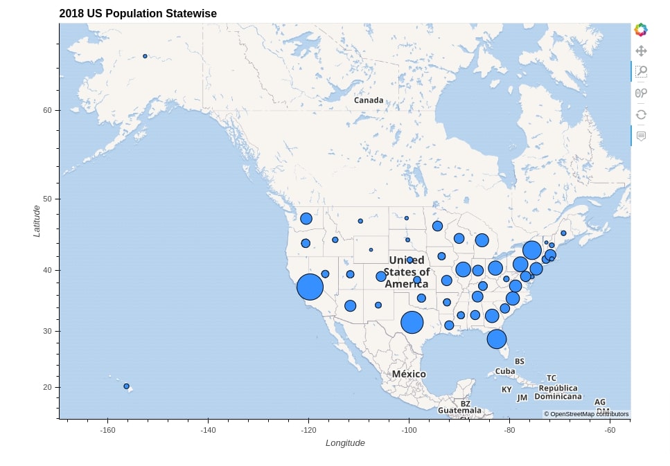
2018 US Population Bubble Map
The first bubble map that we have created shows the population of US states on the US map. In order to create this map, we have loaded and merged a few datasets.
Below we have loaded the first GeoJson dataset which has geometry about the shape of each US state. We have loaded the GeoJSON file using geopandas. The final resulting dataset is geopandas GeoDataFrame where geometry column holds polygon/multi-polygon objects representing individual states of US.
us_states = gpd.read_file("datasets/us-states.json")

us_states.head()
Below we have written a small function named calculate_center() which takes GeoDataFrame as input and returns center of each Polygon/MultiPolygon object present in geometry column of dataframe. We have used this function to retrieve the center of each state of the US. We have also retrieved Longitude and Latitude of the center of each state.
def calculate_center(df):
    """
    Calculate the centre of a geometry

    This method first converts to a planar crs, gets the centroid
    then converts back to the original crs. This gives a more
    accurate
    """
    original_crs = df.crs
    planar_crs = 'EPSG:3857'
    return df['geometry'].to_crs(planar_crs).centroid.to_crs(original_crs)

us_states["center"] = calculate_center(us_states)
us_states["Longitude"] = [val.x for val in us_states.center]
us_states["Latitude"] = [val.y for val in us_states.center]

us_states.head()
Below we have loaded US 2018 population from a CSV file using pandas.
us_pop = pd.read_csv("datasets/State Populations.csv")

us_pop.head()
Now, we have merged the US state’s geo dataframe with the US population dataframe. We have removed geometry and center columns from the resulting dataframe as well. The resulting dataframe will have the population as well as the Longitude and Latitude of the center of each state. We'll be using this final dataframe for creating a bubble map.
us_states_pop = us_states.merge(us_pop, left_on="name", right_on="State").drop(columns=["geometry", "center"])

us_states_pop.head()
At last, we have created a bubble map showing the population of US states in 2018 using Points() method by giving it the merged dataframe that we created earlier. We have set a few options of char using cell magic command and a few using opts() method.
We have merged the points chart with Wikipedia tile to create the final US population bubble map.
%%opts Points [width=900 height=650 title="2018 US Population Statewise" tools=["hover", ]]
%%opts Points (color="dodgerblue" hover_color="lime" line_color="black")

import numpy as np

us_pop_points = geoviews.Points(
                                us_states_pop,
                                kdims=["Longitude", "Latitude"],
                                vdims=["2018 Population", "State"]
                            ).opts(
                                size=np.sqrt(geoviews.dim('2018 Population'))*0.006,
                            )

us_pop_points * geoviews.tile_sources.Wikipedia()
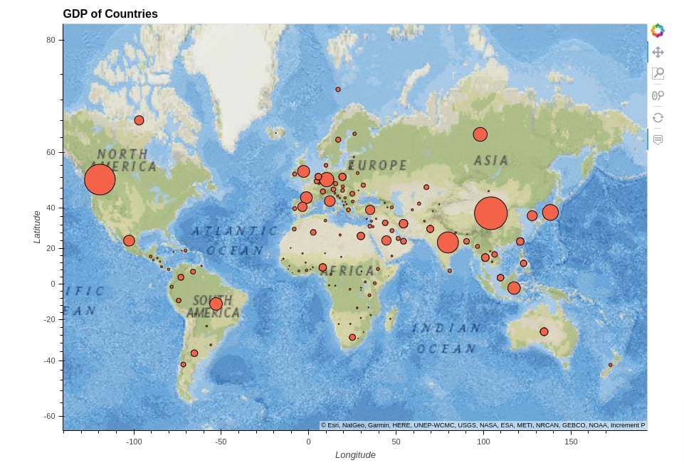
GDP Of World Countries Bubble Map
In this example, we have created a bubble map showing the GDP of various countries on the world map. In order to create this map, we have loaded and merged a few datasets which we'll explain next.
Below we have merged the world geo dataset with the world happiness dataset, both of which we had loaded at the beginning of the tutorial.
world_happiness = world.merge(happiness, left_on="name", right_on="Country or region")

world_happiness.head()
Now, we have retrieved the center of each country of the world using calculate_center() method which we had created earlier. We have also retrieved the longitude and latitude of the center of each country.
world_happiness["center"] = calculate_center(world_happiness)
world_happiness["Longitude"] = [val.x for val in world_happiness.center]
world_happiness["Latitude"] = [val.y for val in world_happiness.center]

world_happiness.head()
Below we have first created bubbles of map using Points() method giving it world happiness merged dataframe which we created in the previous step. While giving the geo dataframe, we have removed geometry and center columns to avoid confusion and errors. We have asked the method to use Longitude and Latitude columns for drawing bubbles and use gdp_md_est column to decide bubble size.
We have set various options of chart using %%opts cell magic command and opts() method.
At last, we have merged the point chart that we created with EsriNatGeo tile to create the final bubble map. The map background comes from the tile.
%%opts Points [width=900 height=650 title="GDP of Countries"]

world_gdp = geoviews.Points(
                                world_happiness.drop(columns=["geometry", "center"]),
                                kdims=["Longitude", "Latitude"],
                                vdims=["Country or region", "gdp_md_est"]
                            ).opts(
                                color="tomato",
                                size=np.sqrt(geoviews.dim('gdp_md_est'))*0.01,
                                tools=["hover",],
                                hover_color="lime",
                                line_color="black"
                            )

world_gdp * geoviews.tile_sources.EsriNatGeo()
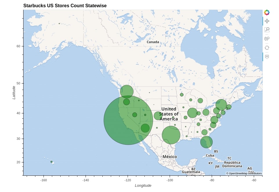
Starbucks US Stores Count Bubble Map
The last bubble map that we'll create will show the number of Starbucks stores per US state. The size of the bubble will be based on the number of stores in that state. In order to create this map, we have modified and merged a few datasets which we have loaded earlier.
First, we have filtered our original Starbucks dataset to keep only entries where the country is the US. We have then retrieved the count of stores per US state by using the grouping functionality of pandas. The final dataframe will have code for each state and store count.
starbucks_us = starbucks[starbucks["Country"] == "US"]

starbucks_us_state_cnt = starbucks_us.groupby("State/Province").count()[["Store Number"]].reset_index().rename(columns={"Store Number":"Store Count"})

starbucks_us_state_cnt.head()
Now we have merged the US state’s geo dataset (US Population Bubble Map Section) which we had created earlier with the state's store count dataset from the previous cell. The resulting merged dataset will have the longitude and latitude of the center of each US state and Starbucks store count as well. We'll be using this dataset for the creation of our last bubble map.
starbucks_us_statewise = us_states_pop.merge(starbucks_us_state_cnt, left_on="id", right_on="State/Province")

starbucks_us_statewise.head()
Below we have first created a bubbles chart using Points() method by giving it a merged dataframe from our previous cell. We have then merged this bubbles chart with Wikipedia tile to bring the map background into the chart. As usual, we have set various chart options using the cell magic command and opts() method.
%%opts Points [width=900 height=650 title="Starbucks US Stores Count Statewise" tools=["hover", ]]
%%opts Points (color="green" hover_color="lime" line_color="black" alpha=0.5)

us_pop_points = geoviews.Points(
                                starbucks_us_statewise,
                                kdims=["Longitude", "Latitude"],
                                vdims=["State", "Store Count"]
                            ).opts(
                                size=geoviews.dim("Store Count") * 0.06,
                            )

us_pop_points * geoviews.tile_sources.Wikipedia()
This ends our small tutorial explaining how we can create scatter and bubble maps using geoviews. Please feel free to let us know your views in the comments section.
References
- Geoviews - Choropleth Maps using Bokeh and Matplotlib
- Getting Started with Holoviews - Basic Interactive Plotting [Python]
- List of Useful Magic Commands in Jupyter Notebook
- Maps using Plotnine (Choropleth, Scatter, and Bubble Maps)
- Choropleth Maps using ipyleaflet [Python]
- Choropleth Maps & Scatter Maps using cufflinks [Python]
- Interactive Choropleth Maps using bqplot [Python]
- Cartopy - Basic Maps [Scatter Map, Bubble Map and Connection Map]
- Plotting Maps using Bokeh [Python]
- ipyleaflet [Python] - Interactive Maps in Python based on leafletjs
- Folium - Interactive Maps [Python]
- How to Create Connection Map Chart in Python Jupyter Notebook [Plotly & Geopandas]?
- hvplot - How to Convert Static Python Maps (Geopandas) to Interactive Maps?
- Geoplot - Scatter & Bubble Maps [Python]
 Sunny Solanki
Sunny Solanki
Intro: Software Developer | Youtuber | Bonsai Enthusiast
About: Sunny Solanki holds a bachelor's degree in Information Technology (2006-2010) from L.D. College of Engineering. Post completion of his graduation, he has 8.5+ years of experience (2011-2019) in the IT Industry (TCS). His IT experience involves working on Python & Java Projects with US/Canada banking clients. Since 2020, he’s primarily concentrating on growing CoderzColumn.
His main areas of interest are AI, Machine Learning, Data Visualization, and Concurrent Programming. He has good hands-on with Python and its ecosystem libraries.
Apart from his tech life, he prefers reading biographies and autobiographies. And yes, he spends his leisure time taking care of his plants and a few pre-Bonsai trees.
Contact: sunny.2309@yahoo.in


![YouTube Subscribe]() Comfortable Learning through Video Tutorials?
Comfortable Learning through Video Tutorials?
If you are more comfortable learning through video tutorials then we would recommend that you subscribe to our YouTube channel.
![Need Help]() Stuck Somewhere? Need Help with Coding? Have Doubts About the Topic/Code?
Stuck Somewhere? Need Help with Coding? Have Doubts About the Topic/Code?
 Stuck Somewhere? Need Help with Coding? Have Doubts About the Topic/Code?
When going through coding examples, it's quite common to have doubts and errors.
If you have doubts about some code examples or are stuck somewhere when trying our code, send us an email at coderzcolumn07@gmail.com. We'll help you or point you in the direction where you can find a solution to your problem.
You can even send us a mail if you are trying something new and need guidance regarding coding. We'll try to respond as soon as possible.
![Share Views]() Want to Share Your Views? Have Any Suggestions?
Want to Share Your Views? Have Any Suggestions?
 Want to Share Your Views? Have Any Suggestions?
If you want to
- provide some suggestions on topic
- share your views
- include some details in tutorial
- suggest some new topics on which we should create tutorials/blogs
 geoviews, scatter-maps, bubble-maps