Cartopy - Basic Maps [Scatter Map, Bubble Map & Connection Map]¶

Table of Contents¶

• Introduction
• 1. First Simple Map
• 2. Trying Different Projections
  • 2.1 PlateCarree Projection
  • 2.2 AlbersEqualArea Projection
  • 2.3 Orthographic Projection
• 3. Adding More Features to Maps
  • 3.1 Adding Coastline, Land, Lakes, Borders, Ocean, Rivers and States Features to Map
  • 3.2 Adding NightShade Feature to Map
• 4. Using Latitude & Longitude Box to Show a Particular Area of Map
• 5. Load Starbucks Locations Dataset
• 6. Scatter Map of Starbucks Locations on Earth [Robinson Projection]
• 7. Scatter Bubble Map depicting Starbucks Store Count Per US States [PlateCarree Projection]
• 8. Loading Brazil Flights Dataset
• 9. Connection Map depicting Flights from Brazil to Other Countries [Mollweide Projection]
• References

Introduction ¶

Many data analysis tasks nowadays involve working with geo spatial data and plot it on maps to get useful insights. For this purpose, we need a trustworthy and reliable plotting library that can be used for plotting maps from a different perspective. Python has a list of libraries (geopandas, bokeh, holoviews, plotly, bqplot, etc) which provides functionalities to plot different types of maps like scatter maps, choropleth map, bubble map, etc. We have already covered tutorials on creating maps using geopandas, holoviews and bqplot.

In this tutorial, we are going to introduce one more python map plotting library named cartopy. Canopy is a map plotting library in python which is based on matplotlib for plotting. It uses PROJ.4, numpy and shapely for handling data conversions between cartographic projection and handling shape files. Cartopy can be very useful to generate a high-quality static map chart that has high publication quality. If you want a high publication chart for your research paper and looking for plotting library with various projections available then cartopy is for you.

The main plus point of cartopy is its object-oriented projection system which lets us plot maps with points, lines polygons, etc using one projection and then can easily let us transfer it to another projection system.

As a part of this tutorial, we'll explore the API of cartopy in order to generate various maps. We'll be using various datasets available from kaggle for our map examples.

We'll start by loading necessary libraries for our plotting purpose.

1. First Simple Map ¶

The generation of maps using cartopy can be done by following below mentioned common steps:

• Create Matplotlib figure using plt.figure().
• Add subplot to figure with projection attribute set as one of the projections available from cartopy.cars module.
• Add features to map like Land, Ocean, Coastline, Borders, etc using cartopy.feature module.
• Add your functionalities like points, lines, etc using common matplotlib API.
• Show plot using plt.show().

Above mentioned steps are common steps when you want to generate world maps but it also provides other functionalities which can let you restrict map area to a particular region. We'll use the above-mentioned steps to plot a simple map.

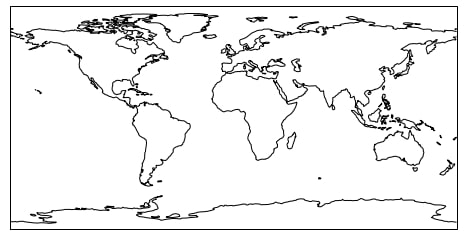
Below we are plotting our first simple plot with projection PlateCarree. We have also added the COASTLINE feature so that we can see all continental borders.

2. Trying Different Projections ¶

We'll now try a few graph projections available in cartopy. The list of projections as available in crs module of the cartopy library.

Full Projections List: https://scitools.org.uk/cartopy/docs/v0.11/crs/projections.html

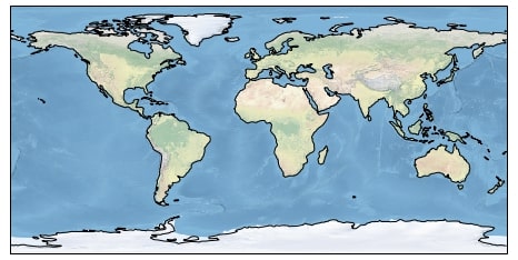
2.1 PlateCarree Projection ¶

Below we are again trying the same PlateCarree projection which we had tried in the previous figure but we have also introduced natural earth look to the plot. We can add it by simply calling the stock_img() method on the axes object. We have also introduced a new way to add new coastline features to our plot.

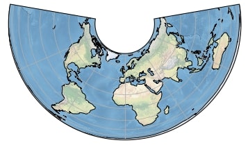
2.2 AlbersEqualArea Projection ¶

Below we have introduced another projection named AlbersEqualArea. We also have introduced grid lines on the plot as a light grey color. The graph generally keeps center at 0 longitudes and 0 latitudes which we can change by setting central_latitude and central_longitude parameter of AlbersEqualArea object.

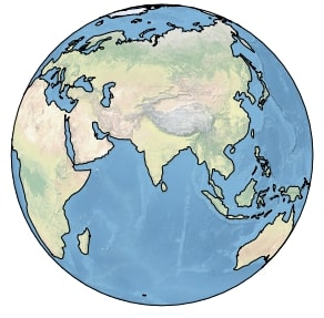
2.3 Orthographic Projection ¶

Below we have introduced another projection named Orthographic which has a shape of the globe. We also have passed its parameter central_latitude and central_longitude which centers glob location on that point which is the center of India.

3. Adding More Features to Maps ¶

We'll now explore further adding more futures to our map plots. Till we only had added coastline features to our maps.

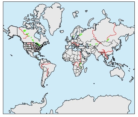
3.1 Adding Coastline, Land, Lakes, Borders, Ocean, Rivers and States Features to Map ¶

Below we are first creating a map with projection as Mercator. We are then adding features by calling method add_feature() on-axis object passing it feature object available from the cartopy.feature module. The list of features available through cartopy is available from the cartopy.feature module.

We are adding below feature to our map:

• COASTLINE feature - Adds coastline around all continents. We can change a coastline color, style, etc.
• LAND feature - Adds land on top of world map. We can change it's color and opacity as well.
• LAKES feature - Adds big lakes of the world. We can change its configuration as well.
• BORDERS feature - Adds country borders for the whole world. We can change border style and color, etc.
• OCEAN feature - Adds ocean with a color that we can change by setting our own configuration as well.
• RIVERS feature - Adds big rivers of the world.
• STATES feature - Adds state boundary for the US.

There are few more classes available from cartopy which lets us add our own designed features but we have not discussed them here as they are not part of the scope of this tutorial.

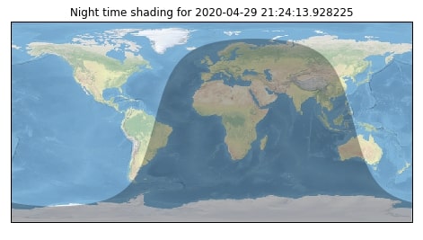
3.2 Adding NightShade Feature to Map ¶

Below we are adding one more feature to cartopy map called nightshade feature. We need to create a datetime object with datetime data and need to pass it to Nightshade object so that it can create nightshade on a map at this time. It'll create a shade effect on a map covering countries where it'll be night during that time.

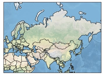
4. Using Latitude & Longitude Box to Show a Particular Area of Map ¶

Below we are explaining how to show only a particular part of the map instead of showing the whole world map. It happens many times that we only need to show a particular country, continent, and region of interest than showing the whole world map. We can do this in two ways:

• We can call method named set_extent() on axes object passing it latitude and longitudes of the area to be covered.
• We can also call set_xlim() and set_ylim() methods passing them longitude and latitude limits respectively.

We have used the below set_extent() method passing it projection as PlateCarree so that it projects box from that projection. We have tried to cover Asia and Europe continents on a map.

We have now explained how to create various maps using cartopy. We'll now explain how to add further more data on maps like plots, lines, etc below. For that, we'll be using the Starbucks store locations dataset and brazil flight dataset.

5. Load Starbucks Locations Dataset ¶

The first dataset that we'll load is Starbucks store locations dataset available from kaggle. We suggest that you download a dataset from kaggle to follow along.

• Stabucks Store Locations Worldwide

This dataset has information about Starbucks store locations worldwide. It has also geospatial information (longitude & latitude) about each store location. Apart from geospatial information, it has data about store address, name, number, ownership type, country, state, city, postcode, etc.

We'll be filtering dataset removing entries from all other countries present other than the United States.

6. Scatter Map of Starbucks Locations on Earth [Robinson Projection] ¶

Below we are plotting scatter map of showing Starbucks locations on the whole Earth.

We have first created a map using a new projection named Robinson. We have then added scatter points on a map using commonly using plt.scatter() the method passing its longitude and latitude of locations. We have also passed it PlateCarree projection as a transform parameter value. We need to pass it so that it plots points on that projection first and then projects it on a map with Robinson projection. This is the convention that we'll be following in future maps as well.

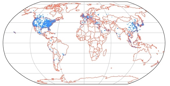
We can notice a high number of Starbucks locations in the whole US and Europe. There is also a sizable number of stores in Chine and Canada as well. All other locations of the world have very less or no Starbucks presence.

7. Scatter Bubble Map depicting Starbucks Store Count Per US States [PlateCarree Projection] ¶

For creating a bubble map of Starbucks store count per US states, we need to prepare data by following the below-mentioned steps.

• We'll first group dataset by State and then take average longitude, latitude for each state
• We'll then group dataset by State and count store counts per state.
• We'll then merge the dataframe created in the previous two steps.

Our final dataset will have an entry for each state along with its latitude, longitude, and Starbucks store count which we'll use for plotting bubble map.

Once we are done with creating a dataset, we'll plot the bubble map exactly the same way as the previous map. We'll call plt.scatter() the method passing it latitude and longitude of each state of the US. We also have passed the size of the marker to be used for each step which is count of stores available in that state. This time we are also restricting graph by setting a limit on it using set_extent() so that it only displays US map. We also have added for states of the US.

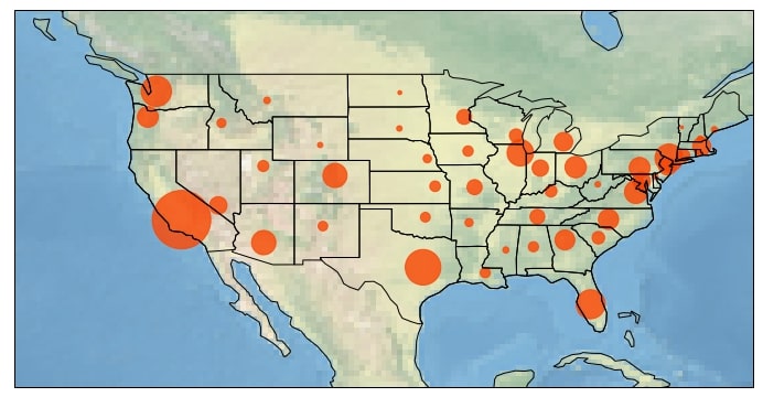
We can notice from the above chart that there is a very high presence of Starbucks in California, Washington, Texas, Florida, Illinois, and New York.

8. Loading Brazil Flights Dataset ¶

The second dataset that we'll be using is flight data for a number of flights from and to Brazil. The dataset is available at kaggle.

• Flights in Brazil

The dataset has information about flight time, type, airline name, source city, destination city, source country, destination country, source state, destination state, source latitude & longitude, and destination latitude & longitude.

We suggest that you download the dataset to follow along with us. Please make a note that the dataset is quite big and has nearly 2.5 Mn rows. If your computer has less memory and wants to follow along with tutorial then we suggest that you load the first few rows only using nrows parameter of read_csv().

9. Connection Map depicting Flights from Brazil to Other Countries [Mollweide Projection] ¶

To plot a connection map depicting flights from Brazil to other countries, we need to first prepare the dataset by following a list of the below steps.

• We'll filter and remove rows where the destination country is Brazil, as well as source and destination country, is Brazil. This way our dataset will have only entries from Brazil to other countries.
• We'll then group dataset by origin & destination country and calculate a count of flights from Brazil to that country.
• We'll then group dataset by origin & destination country, take mean of all columns and then filter the dataset to have only source & destination geospatial data.
• We'll then merge dataset created in the previous two steps to create a final dataset.

Our final dataset will have information about flight count from source to destination countries as well as geospatial data for each country.

Our last map is a connection map where we'll be displaying flight movement from Brazil to various countries of the earth using a line. We also show a thick line where there are more flights going on and a thin line where fewer flights are going.

We have used Mollweide projection this time for the creation of a world map. We are then looping through each flight entry taking the source and destination latitude, longitude to draw line between them using conventional plt.plot() method. We have used Geodetic projection for plotting lines so that it shows a curvy line instead of a straight line from source to destination. We are also plotting names of destination countries where flights are landing from Brazil to highlight them.

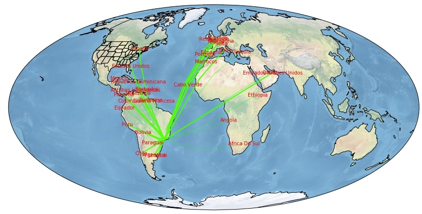
We can sizable number of flight traveling from Brazil to Southern American countries, US, Canada, and European countries. There are some travels to African countries as well but none traveling to Asia.

This ends our small tutorial on covering the basics of cartopy. Please feel free to let us know your views in the comments section.

References ¶

• Plotting Maps using Geopandas
• Interactive Maps using Hvplot (Holoviews)
• Interactive Maps using bqplot
• ipyleaflet - Interactive Maps in Python based on leaflet.js
• Choropleth Maps and Scatter Maps using Cufflinks
• Plotting Maps using Bokeh
• Interactive Choropleth Maps using bqplot
• Choropleth Maps using ipyleaflet
• Connection Maps using Plotly and Geopandas
• Interactive Maps using Folium