Captum: Interpret Predictions Of PyTorch Text Classification Networks¶

Due to tremendous success of deep learning, majority of people have shifted their attention towards designing deep neural networks consisting of different kind of layers to solve machine learning tasks involving unstructured data. The usage of traditional white-box ML models (decision trees, random forests, gradient boosting machines, etc) has decreased over time. Though black-box deep neural networks gives quite good accuracy for tasks based on unstructured datasets, it's quite hard to interpret their predictions. Over the years, many algorithms have been developed to interpret predictions of deep neural networks and many Python libraries (LIME, SHAP, Eli5, Captum, etc.) has been designed that provides implementation of these algorithms.

As a part of this tutorial, we have concentrated on one such Python library named Captum. Captum is designed specifically to interpret predictions of networks designed using PyTorch only. It has implementation of many interpretation algorithms that were invented over the years. Here, we'll use Captum to explain predictions of neural networks that solves text classification tasks. We have listed all available algorithms from Captum in below link. It explains how to use captum for tabular data.

• Captum: Interpret Predictions Of PyTorch Networks (Tabular Data)

If you are looking for guide on using captum for image classification tasks then please check below link.

• Captum for PyTorch Image Classification Networks

Below, we have listed important sections of Tutorial to give an overview of the material covered.

Important Sections Of Tutorial¶

1. Prepare Data
   • 1.1 Load Dataset
   • 1.2 Populate Vocabulary
   • 1.3 Create Data Loaders
2. Define Network
3. Train Network
4. Evaluate Network Performance
5. Explain Predictions using CAPTUM
   • Integrated Gradients
   • Neuron Integrated Gradients

Below, we have imported necessary Python libraries and printed the versions that we have used in our tutorial.

1. Prepare Data ¶

In this section, we are preparing data for neural network. We'll be using word frequency approach for encoding text examples. This approach maintains frequency of words per text example in a vector. We have followed below steps for encoding text data and readying it for neural network.

1. Load Dataset
2. Load through each text example, tokenize them and populate vocabulary of unique tokens (words). The vocabulary is simple mapping from token to integer index. Each token is assigned a unique integer index starting from 0.
3. Vectorize Each text example using populated vocabulary. For each text example, tokenize it and retrieve frequency of each token. The long vector of same size as vocabulary length will be created (per text example) which will have frequency of words at their integer index location as per vocabulary. All other tokens present in vocabulary but not present in text example will have 0 as their frequency.

It is okay if above steps were not clear when you read them. It'll become clear when we actually perform them below.

1.1 Load Dataset¶

In this section, we have loaded our text classification dataset that we are going to use for our task. We'll be using AG NEWS dataset available from datasets module of torchtext Python library. The dataset is already divided into train and test sets. It has text examples for 4 different news categories (["World", "Sports", "Business", "Sci/Tec"]).

1.2 Populate Vocabulary¶

In this section, we have populated vocabulary of unique words using various helper functions available from torchtext library.

First, we have initialized a simple tokenizer using get_tokenizer() function available from torchtext. The tokenizer is a function that takes a text example as input and breaks it into list of words.

text = "Hello, How are you? Where are you planning to go?"
tokenized = ["hello", ",", "how", "are", "you", "?", "where",
            "are", "you", "planning", "to", "go", "?"]

After initializing tokenizer, we have populated a vocabulary using build_vocab_from_iterator() function from vocab module. The function requires an iterator as input which returns list of tokens per each call. We have created a simple function named build_vocabulary() which will work as iterator. It takes as input list of datasets. It then loops through each text examples yielding list of tokens for that example which will be used to populate vocabulary. The vocabulary is simple mapping from word to integer index.

vocab = {
    'hello': 0,
    'how': 1,
    'are': 2,
    'you': 3,
    'where': 4,
    'planning': 5,
    'to': 6,
    'go': 7
    ...
}

After populating vocabulary, we have also printed the size of vocabulary which is number of unique tokens (words) in our datasets.

1.3 Create Data Loaders¶

In this section, we have created data loaders that will be used to loop through data examples in batches during training process.

In order to vectorize each text example using our populated vocabulary from earlier, we have used CountVectorizer class available from scikit-learn. We have created an instance of CountVectorizer using our vocabulary and tokenizer. This vectorizer can take batch of text example as input and returns their vectorized version. The input to CountVectorizer will be of shape (batch_size,) and output will be of shape (batch_size, vocab_len). As we said earlier, for each token of text example, their frequency will be present at their integer index as per vocabulary.

After defining vectorizer, we have created a simple function that takes batch of data (text examples and their target labels) as input and returns vectorized batch data (vectorized examples and target labels). This function will be used by data loaders to vectorize each batch of data.

At last, we have created train and test data loaders using respective datasets. We have set batch size of 256 which will let us loop through data in batches of 256 examples and their labels. We have provided our vectorization function to collate_fn parameter when creating data loaders. This function will be called on each batch of data and its output will be given to network for training.

Below, we have explained with one simple example how vectorization happens.

text = "Hello, How are you? Where are you planning to go?"

vocab = {
    'hello': 0,
    'bye': 1,
    'how': 2,
    'the': 3,
    'welcome': 4,
    'are': 5,
    'you': 6,
    'to': 7
}

vector = [1, 0, 1, 0, 0, 2, 2, 1]

If you are someone who is not aware of word frequency (bag of words) approach of encoding text data and CountVectorizer then we recommend that you go through below link which covers it in detail. It'll help you easily sail through this tutorial.

• Scikit-Learn - Feature Extraction from Text Data

2. Define Network ¶

In this section, we have defined a network that we'll use for our text classification task. The network consist of 3 linear layers with output units 128, 64 and 4 respectively. The last layer has 4 output units which is same as number of target classes. The first layer takes input of shape (batch_size, vocab_len) and outputs processed data of shape (batch_size,128) which is given to second layer for processing. The second layer outputs processed data of shape (batch_size, 64) which is given to third layer for processing. The third layer outputs data of shape (batch_size, 4) which is prediction of network. We have also applied relu activation to the output of first two linear layers. We have created network using Sequential API of PyTorch which is almost same as Keras Sequential API.

After defining network, we have initialized it and performed forward pass through it for verification purposes.

If you are someone who is new to PyTorch and want to learn how to design neural networks using it then please check below link. It'll get you started with the library.

• PyTorch: Simple Guide to Create Neural Networks using "torch.nn" Module

3. Train Network ¶

In this section, we have trained our network. In order to train it, we have designed a function that we'll use to perform training process. The function takes model, loss function, optimizer, train data loader, validation data loader and number of epochs as input. It then executes training loop number of epochs time. For each epoch, it loops through training data in batches. For each batch, it performs forward pass to make predictions, calculates loss, calculates gradients and updates network parameters using gradients. It also prints average loss of all batches of the epoch at the end of epoch. We have also created a helper function to make predictions on validation data and report validation accuracy at the end of each epoch.

Below, we have actually trained our network using function designed in previous cell. We have initialized number of epochs to 5 and learning rate to 0.001. Then, we have initialized our text classification network, Adam optimizer and cross entropy loss function. At last, we have called our training routine with necessary parameters to perform training process. By looking at loss and accuracy values getting printed after each epoch, we can notice that our network is doing a good job at the text classification task.

4. Evaluate Network Performance ¶

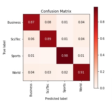
In this section, we have evaluated the performance of our trained network by calculating accuracy score, classification report (precision, recall and f1-score per target class) and confusion matrix metrics on test predictions. We can notice from the test accuracy that our model has done a good job at the given task. We have calculated these metrics using functions available from scikit-learn.

Please feel free to check below link if you are interested in learning various ML metrics available from sklearn.

• Scikit-Learn - Model Evaluation & Scoring Metrics

Apart from calculations, we have also created a visualization for confusion matrix using Python library scikit-plot. The visualization shows that our network is quite good at classifying text documents of Sports category compared to other.

Scikit-plot provides visualizations for many other ML metrics. Please check below link in your free time if you want to learn about them.

• Scikit-Plot: Visualizing Machine Learning Algorithm Results & Performance Metrics

5. Explain Predictions using CAPTUM ¶

In this section, we have explained how we can use Captum to explain predictions made by our network. We'll create visualizations that show which words contributed positively/negatively to prediction. Captum provides many algorithms for explaining predictions but we'll explain a few of them. We suggest that the reader explores further algorithms. All algorithms are available from 'attr' sub-module of captum.

Below, we have simply loaded test text examples and their predictions. We'll randomly select text examples from this dataset and then explain predictions made by our network on these selected examples.

Integrated Gradients¶

In this section, we have explained an algorithm named integrated gradients. This algorithm let us find out the contribution of individual features to the final prediction. The individual features in our case are tokens (words) of our text example.

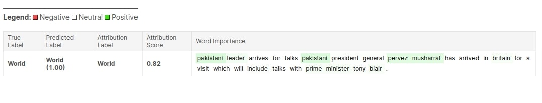
Below, we have first retrieved a random text example from the test dataset and made predictions on it using our trained network. We have printed the actual text of our example, tokenized text, actual label, predicted label, and prediction probabilities. We can notice that our model correctly predicts the target label as 'World' for the selected text example. Now, we'll explain this prediction using integrated gradients algorithm.

In order to explain prediction, we have first created an instance of an algorithm using IntegratedGradients() constructor available from captum. We have provided a function to the constructor that takes a bunch of text examples as input and returns their predictions (softmax probabilities). After initializing the algorithm, we have called attribute() method on it. We have provided a method with vectorized a text example and target label. It returns the contribution of features.

As we have used bag of words (word frequency) approach to vectorize our text examples, each vectorized text example has a length same as the length of vocabulary. It has word frequency at the index location of words from the text example with 0 for all other words not present in the example. Due to this, the feature contributions returned by attribute() method are the same as the length of vocabulary. We have retrieved contributions of words that are present in the text example separately. We can notice the difference in the shape getting printed.

In order to visualize this feature contribution, we need to call visualize_text() method (available from visualization module of captum) with list of VisualizationDataRecord objects. Each VisualizationDataRecord object represents an explanation of one example. We have first created a visualization object with feature contribution, prediction probability, target class, and tokenized text. Then, we have called visualize_text() method with the record to visualize the explanation.

We can notice from the visualization that words like 'pakistani', 'leader', 'minister', 'tony', 'blair', 'britain', etc contribute positively to predicting the target label as 'World'.

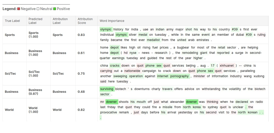
Below, we have retrieved 5 other text examples from the test dataset and made predictions on them using our trained model. We can notice that our model correctly predicts the target label for all of them. We have also printed prediction probabilities for each label. Next, we'll create a visualization explaining all of them using integrated gradients algorithm.

Below, we have generated feature contributions for all text examples and then created visualization data records for them. At last, we have called visualize_text() method with visualization records to create a visualization showing the contribution of words per text example towards the predicted target label. We can notice from the visualization that how words highlighted with green contribute positively towards prediction and words highlighted in red contributes negatively.

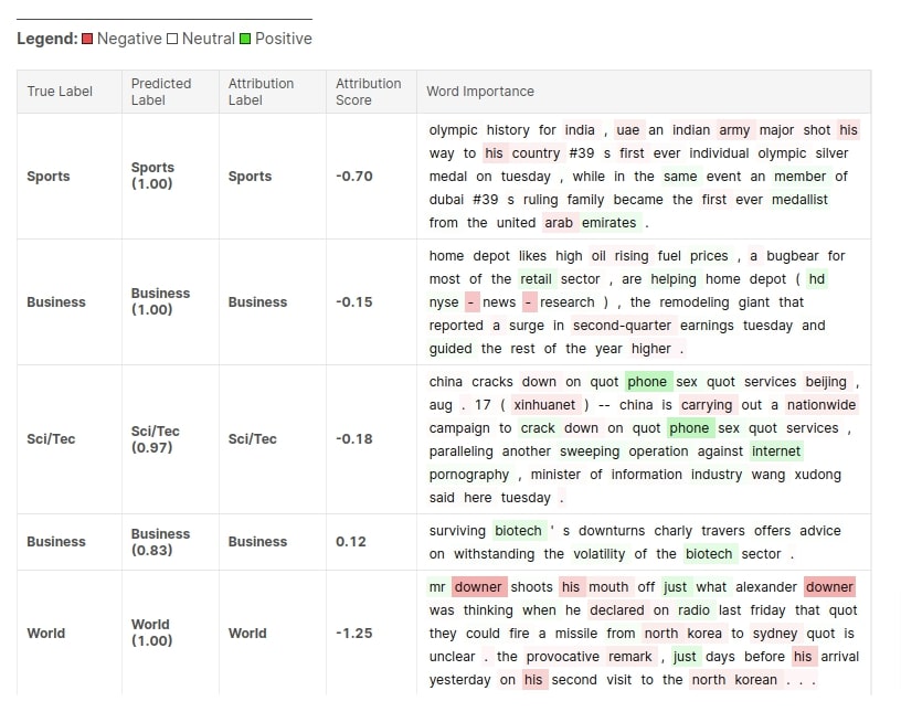
Neuron Integrated Gradients¶

In this section, we have explained the usage of one another algorithms named neuron integrated gradients. This algorithm let us understand the contribution of features toward a particular neuron of the selected layer. This algorithm belongs to the category Neuron Attribution (please check this link to know about algorithm categories in captum).

We have created an instance of an algorithm using NeuronIntegratedGradients() constructor. Apart from the prediction function, this time we have provided reference to the second linear layer as well. When calling attribute() with algorithm, we have provided neuron_selector parameter with value of 0. This will generate features contribution towards activating the 0th neuron of the second linear layer. After generating contributions, we have also visualized them by creating visualization data records.

This ends our small tutorial explaining how we can use captum to explain predictions made by PyTorch network designed for Text Classification tasks. Please feel free to contact us to let us know your views.

References¶

LIME Tutorials¶

• How to Use LIME to Understand sklearn Models Predictions?
• LIME: Interpret Predictions Of Flax (JAX) Text Classification Networks
• LIME: Interpret Predictions Of Keras Text Classification Networks

SHAP Values Tutorials¶

• SHAP - Explain Machine Learning Model Predictions using Game Theoretic Approach
• Explain Text Classification Models Using SHAP Values (Keras + Vectorized Data)
• Explain Flax (JAX) Text Classification Networks using SHAP Values

Eli5 Tutorials¶

• How to Use eli5 to Understand sklearn Models, their Performance, and their Predictions?
• Eli5.lime: Explain PyTorch Text Classification Network Predictions Using LIME Algorithm
• Eli5.lime: Explain Flax (JAX) Text Classifier Predictions Using LIME

Other Libraries¶

• interpret-text - Interpret NLP Models and Their Predictions
• Yellowbrick - Text Data Visualizations