Captum: Interpret Predictions Of PyTorch Image Classification Networks
With the rise of deep learning, neural networks have become deeper and deeper with different types of layers (Convolution, Recurrent, LSTM, ConvLSTM, etc.) to transform data and find out patterns. Though this deep neural network gives the best results, especially for unstructured data (image, text, audio, etc), they are super hard to interpret. The predictions made by traditional ML models (decision trees, random forests, gradient boosting machines, etc) which are generally considered white-box models are fairly simple to interpret. Still, they do not perform well for unstructured data. Interpretability is a very important aspect of a network's performance evaluation as we want to know why our model is making a particular prediction and what parts of the data are contributing to that prediction. If our image classification network classifying cat vs dog is giving 95%+ accuracy then we want to know that it is using pixels of an image where either cat or dog are present to make predictions and not using some background pixels for predictions. Though interpreting predictions of deep neural networks (black-box models) is hard, over time, many algorithms have been developed to tackle the task.
As a part of this tutorial, we have explained a library called Captum which is specifically designed to interpret/explain predictions of neural networks designed using PyTorch. It provides an implementation for the majority of interpretation algorithms that have been invented till now. It'll keep adding more algorithms as they are introduced. In this tutorial, we have designed a simple convolutional neural network using PyTorch for image classification tasks. We'll use captum to explain predictions made by this network.
We have already covered the basics of captum and listed all available algorithms in a separate started tutorial. Please feel free to check it in your free time as it'll get you started with the library if you are new to it. It explains the library usage over tabular datasets.
Below, we have listed important sections of tutorial to give an overview of the material covered.
Important Sections Of Tutorial
- Load Dataset
- Define Network
- Train Network
- Evaluate Network Performance
- Explain Network Predictions using CAPTUM
- Primary Attribution
- Integrated Gradients
- Gradient SHAP
- Guided Grad-CAM
- DeepLIFT
- Kernel SHAP
- Layer Attribution
- Grad-CAM
- Layer DeepLIFT
- Layer Integrated Gradients
- Neuron Attribution
- Neuron Gradient
- Neuron Integrated Gradients
- Neuron Gradient SHAP
- Primary Attribution
Below, we have imported the necessary Python libraries and printed the versions we used in our tutorial.
import torch

print("Torch Version : {}".format(torch.__version__))
import torchvision

print("Torch Vision Version : {}".format(torchvision.__version__))
import captum

print("Captum Version : {}".format(captum.__version__))
1. Load Dataset 
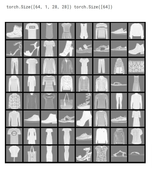
In this section, we have loaded Fashion MNIST dataset that we are going to use for our classification task. The dataset has grayscale images of shape (28,28) pixels for 10 different fashion items. The dataset is available from datasets module of torchvision Python library. The dataset is already divided into the train (60k images) and test (10k images) sets. After loading datasets, we have created data loaders from them which will be used to go through data in batches during the training process. The batch size of 64 is used. Below, we have included a table of mapping from target class index to target class name.
| Label | Description |
|---|---|
| 0 | T-shirt/top |
| 1 | Trouser |
| 2 | Pullover |
| 3 | Dress |
| 4 | Coat |
| 5 | Sandal |
| 6 | Shirt |
| 7 | Sneaker |
| 8 | Bag |
| 9 | Ankle boot |
from torchvision.datasets import CIFAR10, FashionMNIST
from torch.utils.data import DataLoader
from torchvision import transforms, utils as vis_utils

img_transforms = transforms.Compose([transforms.ToTensor(),])
                                     #transforms.Normalize((0.5, 0.5, 0.5), (0.5, 0.5, 0.5))])

fmnist_train_dataset = FashionMNIST(root=".",train=True, download=True, transform=img_transforms)
fmnist_test_dataset  = FashionMNIST(root=".",train=False, download=True, transform=img_transforms)

train_loader = DataLoader(fmnist_train_dataset, batch_size=64)
test_loader = DataLoader(fmnist_test_dataset, batch_size=64)

len(train_loader), len(test_loader)
fmnist_train_dataset.classes
After loading datasets and creating data loaders, we have plotted a few sample images for reference purposes below.
import matplotlib.pyplot as plt
import torchvision.transforms.functional as vis_F

batch_size, n_channels, height, width = [None] * 4
for X, Y in train_loader:
    print(X.shape, Y.shape)
    batch_size, n_channels, height, width = X.shape
    plt.figure(figsize=(9,9))
    plt.imshow(vis_F.to_pil_image(vis_utils.make_grid(X/2 + 0.5)));
    plt.xticks([],[]); plt.yticks([],[]);
    break
batch_size, n_channels, height, width
2. Define Network 
In this section, we have defined a network that we'll use for our image classification task. The network consists of 2 convolution layers and one linear layer. The first convolution layer has 32 output channels and applies kernel of shape (3,3) on input data. The second convolution layer has 16 output channels and applies kernel of shape (3,3) on input data. The relu activation is applied to the output of both convolution layers. The output of the second convolution layer is given to the linear layer that has 10 output units. The output of the linear layer is a prediction of network. We have defined our network using Sequential API of PyTorch which is almost the same as Keras Sequential API.
After defining the network, we initialized it and performed a forward pass using a few examples for verification purposes.
If you are new to PyTorch and looking for guidance on creating neural networks then please feel free to check the below links. It'll get you started with the library.
from torch import nn
from torch.nn import functional as F

class Classifier(nn.Module):
    def __init__(self):
        super(Classifier, self).__init__()
        self.seq = nn.Sequential(
            #nn.Conv2d(3, 64, kernel_size=(3,3), padding="same", padding_mode="zeros"),
            #nn.ReLU(),

            nn.Conv2d(n_channels, 32, kernel_size=(3,3), padding="same", padding_mode="zeros"),
            nn.ReLU(),

            nn.Conv2d(32, 16, kernel_size=(3,3), padding="same", padding_mode="zeros"),
            nn.ReLU(),

            nn.Flatten(),
            nn.Linear(16*height*width, len(fmnist_train_dataset.classes)),
            #nn.Softmax(dim=1)
        )

    def forward(self, X_batch):
        return self.seq(X_batch)

classifier = Classifier()

classifier
preds = classifier(X)

preds.shape
3. Train Network 
In this section, we are training the network that we designed in the previous cell. In order to train the network, we have defined a function. The function takes model, loss function, optimizer, train data loader, validation data loader, and a number of epochs as input. The function executes training loop number of epochs times. For each epoch, it loops through training data in batches. For each batch of data, it performs a forward pass to make predictions, calculates loss, calculates gradients, and updates network parameters using gradients. It records loss for each batch and prints the average training loss at the end of each epoch. We have also created other helper functions that calculate validation loss and accuracy.
from sklearn.metrics import accuracy_score
from tqdm import tqdm
import gc

def CalcValLoss(model, loss_func, val_loader):
    with torch.no_grad(): ## Prevents calculation of gradients
        val_losses = []
        for X_batch, Y_batch in val_loader:
            preds = model(X_batch)
            loss = loss_func(preds, Y_batch)
            val_losses.append(loss)
        print("Valid CategoricalCrossEntropy : {:.3f}".format(torch.tensor(val_losses).mean()))

def MakePredictions(model, loader):
    preds, Y_shuffled = [], []
    for X_batch, Y_batch in loader:
        preds.append(model(X_batch))
        Y_shuffled.append(Y_batch)

    preds = torch.cat(preds).argmax(axis=-1)
    Y_shuffled = torch.cat(Y_shuffled)
    return Y_shuffled, preds

def TrainModelInBatchesV1(model, loss_func, optimizer, train_loader, val_loader, epochs=5):
    for i in range(epochs):
        losses = [] ## Record loss of each batch
        for X_batch, Y_batch in tqdm(train_loader):
            preds = model(X_batch) ## Make Predictions by forward pass through network

            loss = loss_func(preds, Y_batch) ## Calculate Loss
            losses.append(loss) ## Record Loss

            optimizer.zero_grad() ## Zero weights before calculating gradients
            loss.backward() ## Calculate Gradients
            optimizer.step() ## Update Weights
            gc.collect()

        print("Train CategoricalCrossEntropy : {:.3f}".format(torch.tensor(losses).mean()))
        CalcValLoss(model, loss_func, val_loader)

        Y_test_shuffled, test_preds = MakePredictions(model, val_loader)
        val_acc = accuracy_score(Y_test_shuffled, test_preds)
        print("Val  Accuracy : {:.3f}".format(val_acc))
        gc.collect()
Below, we have trained our network using a function defined in the previous cell. We have first initialized a number of epochs to 8 and the learning rate to 0.001. Then, we have initialized the classification model, cross entropy loss, and Adam optimizer. At last, we have called our training routine with the necessary parameters to perform the training process. We can notice from the loss and accuracy values getting printed after each epoch that our network is doing a good job at the image classification task.
from torch.optim import SGD, RMSprop, Adam

#torch.manual_seed(42) ##For reproducibility.This will make sure that same random weights are initialized each time.
epochs = 8
learning_rate = torch.tensor(1e-3) # 0.001

classifier = Classifier()
cross_entropy_loss = nn.CrossEntropyLoss()
optimizer = Adam(params=classifier.parameters(), lr=learning_rate)

TrainModelInBatchesV1(classifier, cross_entropy_loss, optimizer, train_loader, test_loader,epochs)
4. Evaluate Network Performance 
In this section, we have evaluated the performance of our trained network by calculating accuracy score, classification report (precision, recall, and f1-score per target class) and confusion matrix ML metrics on test predictions. We can notice from the accuracy score that the network is doing an above-average job at the task. We have calculated these metrics using functions available from scikit-learn.
Please feel free to check the below link if you are interested in learning about various ML metrics available from sklearn.
Apart from calculations, we have also created a visualization of the confusion matrix using Python library scikit-plot. The visualization highlights that our network is not good at classifying images of target categories Pullover and Shirt. Many shirts are confused with T-shirts. Pullovers are confused with coats very often.
Scikit-plot provides visualization for many other ML metrics. Please check the below link if you are interested in it.
from sklearn.metrics import accuracy_score, classification_report, confusion_matrix

Y_test_shuffled, test_preds = MakePredictions(classifier, test_loader)

print("Test  Accuracy : {:.3f}".format(accuracy_score(Y_test_shuffled, test_preds)))
print("\nTest Data Classification Report : ")
print(classification_report(Y_test_shuffled, test_preds, target_names=fmnist_train_dataset.classes))
print("\nTest Data Confusion Matrix : ")
print(confusion_matrix(Y_test_shuffled, test_preds))
import scikitplot as skplt
import matplotlib.pyplot as plt

skplt.metrics.plot_confusion_matrix([fmnist_train_dataset.classes[i] for i in Y_test_shuffled], [fmnist_train_dataset.classes[i] for i in test_preds],
                                    normalize=True,
                                    title="Confusion Matrix",
                                    cmap="Oranges",
                                    hide_zeros=True,
                                    figsize=(8,8)
                                    );
plt.xticks(rotation=90);

5. Explain Network Predictions using CAPTUM 
Now, we'll explain predictions made by our network using Python library captum. It provides an implementation for many famous interpretation algorithms. Captum divides algorithms into 3 categories.
- Primary Attribution - The algorithms in this category let us find out the contribution of our input data features towards prediction. (Input Features --> Prediction)
- Layer Attribution - The algorithms in this category let us find out the contribution of activations of the selected layer towards prediction. (Layer Activations --> Prediction)
- Neuron Attribution - The algorithms in this category let us find out the contributions of input data features towards the activation of a particular neuron. (Input Features --> Neuron Activation)
We'll explain the usage of a few algorithms from each category. All algorithms are available from 'attr' sub-module of captum. If the reader is interested in the theory of algorithms then we recommend going through the below link that covers them all in detail.
1. Primary Attribution
In this section, we'll explain a few algorithms from Primary Attribution category. Below, we have retrieved a few images and their target labels from the test data loader. Then, we made predictions on the first image using our trained model. We have printed the actual label and predicted label for reference purposes. Our network correctly predicts the target label as Ankle Boot. Next, we'll interpret this prediction and find out which features contributed to it.
X, Y = iter(test_loader).next()
Y_logits = classifier(X)
Y_probs = F.softmax(Y_logits, dim=-1)
Y_preds = Y_probs.argmax(axis=-1)

print("Actual        : {}".format(fmnist_train_dataset.classes[Y[0]]))
print("Prediction    : {}".format(fmnist_train_dataset.classes[Y_preds[0]]))
print("Probabilities : {}".format(dict(zip(fmnist_train_dataset.classes,Y_probs[0].detach().numpy()))))
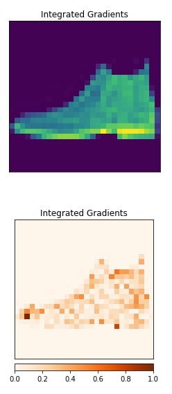
Integrated Gradients
In this section, we have explained the usage of integrated gradients algorithm. We have created an instance of algorithm using IntegratedGradients() constructor available from 'attr' sub-module of captum. We have given our PyTorch network to the constructor. In order to generate an explanation for prediction, we need to call attribute() method. We have called the method with the first image and its target label. The output is an interpretation. Here, we have given only one grayscale image hence shape is (1,1,28,28) but you can give as many as you want. This returned image is a kind of mast that highlights pixels that contributed to predicting the target label as Ankle Boot.
Next, we have visualized original image and returned explanation using visualize_image_attr() function available from 'visualization' sub-module of 'attr'. The method uses Python library matplotlib to generate visualizations. We can notice from the explanation image that pixels present in the ankle boot section are contributing to prediction which is good. If this returns pixels other than object pixels (for example background pixels) then we can consider that our model has not generalized well.
Please make a NOTE that we have reshaped images before giving them to the visualization method as matplotlib requires channels at last and we had channels at the beginning.
from captum.attr import IntegratedGradients

classifier.eval()

algorithm = IntegratedGradients(classifier)

feature_imp_img = algorithm.attribute(X[:1], target=Y[:1])

feature_imp_img.shape
import numpy as np
from captum.attr import visualization as viz

orig_image = np.transpose(X[0].numpy(), (1,2,0))

viz.visualize_image_attr(None, orig_image, method="original_image",
                         title="Integrated Gradients",fig_size=(4,4));
viz.visualize_image_attr(feature_imp_img.numpy().reshape(28,28,1), orig_image,
                         show_colorbar=True, cmap="Oranges", title="Integrated Gradients", fig_size=(4,4));
#viz.visualize_image_attr(feature_imp_img.numpy().reshape(28,28,1), orig_image, method="blended_heat_map", show_colorbar=True, cmap="Oranges", title="Integrated Gradients");
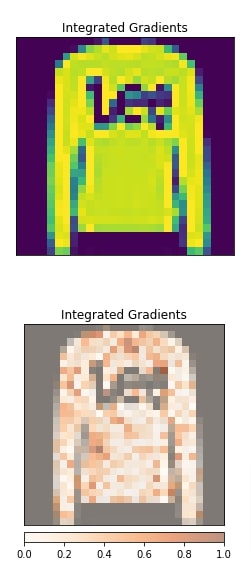
Gradient SHAP
In this section, we have explained the usage of gradient shap algorithm. We have selected a different image this time. The selected image is Pullover and our network correctly predicts the target label. Our model has little low prediction probability for this prediction.
print("Actual        : {}".format(fmnist_train_dataset.classes[Y[1]]))
print("Prediction    : {}".format(fmnist_train_dataset.classes[Y_preds[1]]))
print("Probabilities : {}".format(dict(zip(fmnist_train_dataset.classes,Y_probs[1].detach().numpy()))))
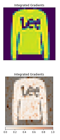
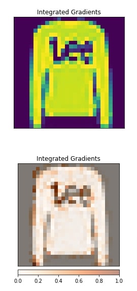
We have created an algorithm using the constructor GradientShap(). We have generated an explanation for the second image from our data and then visualized it. We can notice from the visualization that pixels inside of the pullover are contributing to prediction.
from captum.attr import GradientShap

algorithm = GradientShap(classifier)

feature_imp_img = algorithm.attribute(X[1:2], target=Y[1:2], baselines=torch.zeros_like(X[:1]))

feature_imp_img.shape
import numpy as np
from captum.attr import visualization as viz

orig_image = np.transpose(X[1].numpy(), (1,2,0))

viz.visualize_image_attr(None, orig_image, method="original_image", title="Integrated Gradients",fig_size=(4,4));
viz.visualize_image_attr(feature_imp_img.numpy().reshape(28,28,1), orig_image, method="blended_heat_map",
                         show_colorbar=True, cmap="Oranges", title="Integrated Gradients", fig_size=(4,4));
Guided Grad-CAM
In this section, we have explained the usage of Guide Grad-CAM algorithm. This algorithm requires reference to the convolution layer of the network and produces an explanation with respect to that layer.
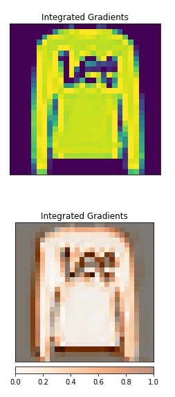
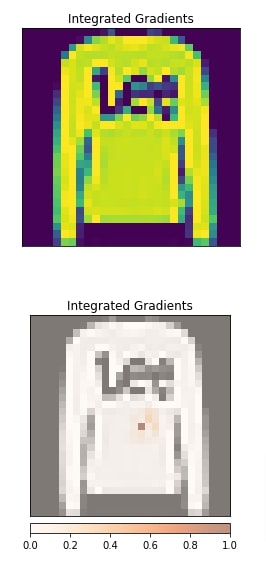
We have created an algorithm using GuidedGradCam() constructor. We have provided reference to the second convolution layer. After generating an explanation, we have plotted it as usual. The visualization indicates that the second convolution layer seems to be detecting an edge of the pullover.
layers = list(classifier.modules())[2:]

layers
from captum.attr import GuidedGradCam

algorithm = GuidedGradCam(classifier, layer=layers[2])

feature_imp_img = algorithm.attribute(X[1:2], target=Y[1:2])

feature_imp_img.shape
import numpy as np
from captum.attr import visualization as viz

orig_image = np.transpose(X[1].numpy(), (1,2,0))

viz.visualize_image_attr(None, orig_image, method="original_image", title="Integrated Gradients",fig_size=(4,4));
viz.visualize_image_attr(feature_imp_img.detach().numpy().reshape(28,28,1), orig_image, method="blended_heat_map",
                         show_colorbar=True, cmap="Oranges", title="Integrated Gradients", fig_size=(4,4));
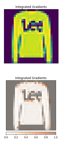
DeepLIFT
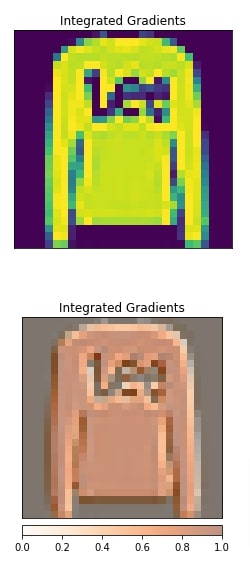
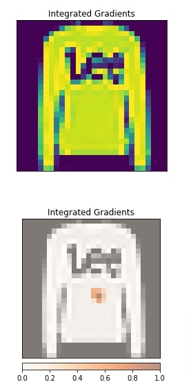
In this section, we have generated an explanation using DeepLIFT algorithm. The algorithm is created using DeepLift() constructor. The visualization shows that pixels in the pullover seem to be contributing to prediction.
from captum.attr import DeepLift

algorithm = DeepLift(classifier)#, layer=layers[2])

feature_imp_img = algorithm.attribute(X[1:2], target=Y[1:2])

feature_imp_img.shape
import numpy as np
from captum.attr import visualization as viz

orig_image = np.transpose(X[1].numpy(), (1,2,0))

viz.visualize_image_attr(None, orig_image, method="original_image", title="Integrated Gradients",fig_size=(4,4));
viz.visualize_image_attr(feature_imp_img.detach().numpy().reshape(28,28,1), orig_image, method="blended_heat_map",
                         show_colorbar=True, cmap="Oranges", title="Integrated Gradients", fig_size=(4,4));

Kernel SHAP
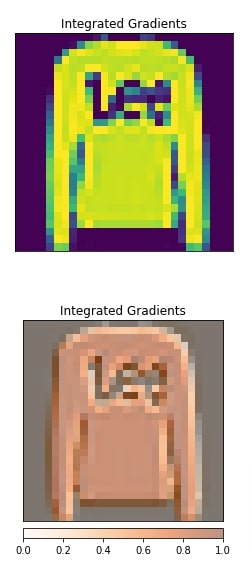
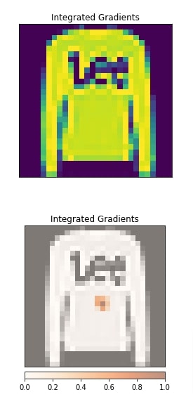
In this section, we have generated an explanation using kernel SHAP algorithm. The algorithm is initialized using KernelShap() constructor. The visualization shows that other than pullover pixels some background pixels are also contributing to prediction which is not good. This can happen because our model is already weak at classifying pullovers and it predicted our selected pullover correct with less probability.
from captum.attr import KernelShap

algorithm = KernelShap(classifier)#, layer=layers[2])

feature_imp_img = algorithm.attribute(X[1:2], target=Y[1:2])

feature_imp_img.shape
import numpy as np
from captum.attr import visualization as viz

orig_image = np.transpose(X[1].numpy(), (1,2,0))

viz.visualize_image_attr(None, orig_image, method="original_image", title="Integrated Gradients",fig_size=(4,4));
viz.visualize_image_attr(feature_imp_img.detach().numpy().reshape(28,28,1), orig_image, method="blended_heat_map",
                         show_colorbar=True, cmap="Oranges", title="Integrated Gradients", fig_size=(4,4));
2. Layer Attribution
In this section, we'll explain network predictions using Layer Attribution algorithms. The algorithms in this section require us to provide a reference layer from which to generate an explanation. All algorithms from this category start with the string 'Layer' to differentiate them from other categories.
Grad-CAM
In this section, we have explained the usage of Grad-CAM algorithm. We have instantiated algorithm using LayerGradCam() constructor. We have provided a classification model and second convolution layer to the constructor. Then, we have created an explanation using attribute() method and visualized it along with the original image for comparison purposes. We can notice from the visualization that the second convolution layer seems to detect the edges of images.
layers = list(classifier.modules())[2:]

layers
from captum.attr import LayerGradCam

algorithm = LayerGradCam(classifier, layer=layers[2])

feature_imp_img = algorithm.attribute(X[1:2], target=Y[1:2])

feature_imp_img.shape
import numpy as np
from captum.attr import visualization as viz

orig_image = np.transpose(X[1].numpy(), (1,2,0))

viz.visualize_image_attr(None, orig_image, method="original_image", title="Integrated Gradients",fig_size=(4,4));
viz.visualize_image_attr(feature_imp_img.detach().numpy().reshape(28,28,1), orig_image, method="blended_heat_map",
                         show_colorbar=True, cmap="Oranges", title="Integrated Gradients", fig_size=(4,4));
Below, we have generated an explanation with respect to the first convolution layer. We can notice from the visualization that it also seems to detect edges along with internal pixels.
from captum.attr import LayerGradCam

algorithm = LayerGradCam(classifier, layer=layers[0])

feature_imp_img = algorithm.attribute(X[1:2], target=Y[1:2])

feature_imp_img.shape
import numpy as np
from captum.attr import visualization as viz

orig_image = np.transpose(X[1].numpy(), (1,2,0))

viz.visualize_image_attr(None, orig_image, method="original_image", title="Integrated Gradients",fig_size=(4,4));
viz.visualize_image_attr(feature_imp_img.detach().numpy().reshape(28,28,1), orig_image, method="blended_heat_map",
                         show_colorbar=True, cmap="Oranges", title="Integrated Gradients", fig_size=(4,4));
Layer DeepLIFT
In this section, we have created an explanation using Layer DeepLIFT algorithm with respect to the first convolution layer. The visualization highlights that the results are almost the same as the previous Grad-CAM algorithm.
from captum.attr import LayerDeepLift

algorithm = LayerGradCam(classifier, layer=layers[0])

feature_imp_img = algorithm.attribute(X[1:2], target=Y[1:2])

feature_imp_img.shape
import numpy as np
from captum.attr import visualization as viz

orig_image = np.transpose(X[1].numpy(), (1,2,0))

viz.visualize_image_attr(None, orig_image, method="original_image", title="Integrated Gradients",fig_size=(4,4));
viz.visualize_image_attr(feature_imp_img.detach().numpy().reshape(28,28,1), orig_image, method="blended_heat_map",
                         show_colorbar=True, cmap="Oranges", title="Integrated Gradients", fig_size=(4,4));
Layer Integrated Gradients
In this section, we have created an explanation using Layer integrated algorithms with respect to the first convolution layer. We can notice from the visualization that the second convolution layer is making a few edge pixels and a few middle pixels contribute towards prediction.
from captum.attr import LayerIntegratedGradients

algorithm = LayerIntegratedGradients(classifier, layer=layers[0])

feature_imp_img = algorithm.attribute(X[1:2], target=Y[1:2])

feature_imp_img.shape
feature_imp_img = feature_imp_img.mean(axis=1)

feature_imp_img.shape
import numpy as np
from captum.attr import visualization as viz

orig_image = np.transpose(X[1].numpy(), (1,2,0))

viz.visualize_image_attr(None, orig_image, method="original_image", title="Integrated Gradients",fig_size=(4,4));
viz.visualize_image_attr(feature_imp_img.detach().numpy().reshape(28,28,1), orig_image, method="blended_heat_map",
                         show_colorbar=True, cmap="Oranges", title="Integrated Gradients", fig_size=(4,4));
3. Neuron Attribution
In this section, we have explained how to use algorithms from Neuron Attribution category. The algorithms in this category require us to provide a reference layer and neuron index as it lets us know input data features contribute to the activation of that neuron. All algorithms from this category start with the string 'Neuron' to differentiate them from other categories.
layers
Neuron Gradient
In this section, we have generated an explanation using Neuron gradient algorithm. We have initialized the algorithm using NeuronGradient() constructor. We have provided a classification network and the first convolution layer to the constructor. When calling attribute() method for algorithms in this section, we need to provide a neuron index. The output of second convolution layer has shape of (batch_size,32,28,28) hence per example there are (32,28,28) = (channels, height, width) activated neurons. We need to provide a tuple of 3 values to index a neuron. We have selected neuron at (0,15,15) which points at the first channel, 16th pixel in height dimension, and 16th pixel in the width dimension.
After generating an explanation, we have visualized it as well. We can notice from visualization the contribution of features towards the activation of that neuron.
from captum.attr import NeuronGradient

algorithm = NeuronGradient(classifier, layer=layers[0])

feature_imp_img = algorithm.attribute(X[1:2], neuron_selector=(0,15,15)) ## (output_channels, height, width)

feature_imp_img.shape
import numpy as np
from captum.attr import visualization as viz

orig_image = np.transpose(X[1].numpy(), (1,2,0))

viz.visualize_image_attr(None, orig_image, method="original_image", title="Integrated Gradients",fig_size=(4,4));
viz.visualize_image_attr(feature_imp_img.detach().numpy().reshape(28,28,1), orig_image, method="blended_heat_map",
                         show_colorbar=True, cmap="Oranges", title="Integrated Gradients", fig_size=(4,4));
Neuron Integrated Gradients
In this section, we have explained the usage of neuron integrated gradients. The algorithm is initiated using NeuronIntegratedGradients() constructor. The explanation is created with respect to neuron at position (0,15,15) in the first convolution layer. After generating an explanation, we have visualized it as well.
from captum.attr import NeuronIntegratedGradients

algorithm = NeuronIntegratedGradients(classifier, layer=layers[0])

feature_imp_img = algorithm.attribute(X[1:2], neuron_selector=(0,15,15))  ## (output_channels, height, width)

feature_imp_img.shape
import numpy as np
from captum.attr import visualization as viz

orig_image = np.transpose(X[1].numpy(), (1,2,0))

viz.visualize_image_attr(None, orig_image, method="original_image", title="Integrated Gradients",fig_size=(4,4));
viz.visualize_image_attr(feature_imp_img.detach().numpy().reshape(28,28,1), orig_image, method="blended_heat_map",
                         show_colorbar=True, cmap="Oranges", title="Integrated Gradients", fig_size=(4,4));
Neuron Gradient SHAP
In this section, we have explained the usage of neuron gradient SHAP algorithm. The algorithm is initiated using NeuronGradientShap() constructor. We have generated input data features contribution with respect to the neuron at position (15,15,15) from the second convolution layer. After generating an explanation, we have visualized it as well.
from captum.attr import NeuronGradientShap

algorithm = NeuronGradientShap(classifier, layer=layers[2])

feature_imp_img = algorithm.attribute(X[1:2], neuron_selector=(15,15,15),
                                      baselines=torch.zeros_like(X[1:2])) ## (output_channels, height, width)

feature_imp_img.shape
import numpy as np
from captum.attr import visualization as viz

orig_image = np.transpose(X[1].numpy(), (1,2,0))

viz.visualize_image_attr(None, orig_image, method="original_image", title="Integrated Gradients",fig_size=(4,4));
viz.visualize_image_attr(feature_imp_img.detach().numpy().reshape(28,28,1), orig_image, method="blended_heat_map",
                         show_colorbar=True, cmap="Oranges", title="Integrated Gradients", fig_size=(4,4));
This ends our small tutorial explaining how we can use various interpretation algorithms available from Captum to interpret predictions of PyTorch Image classification networks.
References
LIME Tutorials
- How to Use LIME to Understand sklearn Models Predictions?
- LIME: Explain Keras Image Classification Network (CNN) Predictions
SHAP Values Tutorials
- SHAP - Explain Machine Learning Model Predictions using Game Theoretic Approach
- SHAP Values for Image Classification Tasks (Keras)
- Explain Flax (JAX) Image Classification Network Predictions using SHAP Values
Eli5 Tutorials
- How to Use eli5 to Understand sklearn Models, their Performance, and their Predictions?
- Eli5: Explain Image Classifier Predictions Using Grad-CAM (Keras)
Grad-CAM Implementations
 Sunny Solanki
Sunny Solanki
Intro: Software Developer | Youtuber | Bonsai Enthusiast
About: Sunny Solanki holds a bachelor's degree in Information Technology (2006-2010) from L.D. College of Engineering. Post completion of his graduation, he has 8.5+ years of experience (2011-2019) in the IT Industry (TCS). His IT experience involves working on Python & Java Projects with US/Canada banking clients. Since 2020, he’s primarily concentrating on growing CoderzColumn.
His main areas of interest are AI, Machine Learning, Data Visualization, and Concurrent Programming. He has good hands-on with Python and its ecosystem libraries.
Apart from his tech life, he prefers reading biographies and autobiographies. And yes, he spends his leisure time taking care of his plants and a few pre-Bonsai trees.
Contact: sunny.2309@yahoo.in


![YouTube Subscribe]() Comfortable Learning through Video Tutorials?
Comfortable Learning through Video Tutorials?
If you are more comfortable learning through video tutorials then we would recommend that you subscribe to our YouTube channel.
![Need Help]() Stuck Somewhere? Need Help with Coding? Have Doubts About the Topic/Code?
Stuck Somewhere? Need Help with Coding? Have Doubts About the Topic/Code?
 Stuck Somewhere? Need Help with Coding? Have Doubts About the Topic/Code?
When going through coding examples, it's quite common to have doubts and errors.
If you have doubts about some code examples or are stuck somewhere when trying our code, send us an email at coderzcolumn07@gmail.com. We'll help you or point you in the direction where you can find a solution to your problem.
You can even send us a mail if you are trying something new and need guidance regarding coding. We'll try to respond as soon as possible.
![Share Views]() Want to Share Your Views? Have Any Suggestions?
Want to Share Your Views? Have Any Suggestions?
 Want to Share Your Views? Have Any Suggestions?
If you want to
- provide some suggestions on topic
- share your views
- include some details in tutorial
- suggest some new topics on which we should create tutorials/blogs
 captum, pytorch, interpretation, image-classification