Updated On : Feb-28,2022 Time Investment : ~30 mins

Explain Flax (JAX) Image Classification Network Predictions using SHAP Values¶

The latest advancement in deep learning has increased the accuracy of many computer vision problems like image classification. Now, it's possible to get good accuracy for image classification tasks using even simple convolution neural networks. Though it is possible to get good accuracy with image classification tasks, we need to understand how our model is making predictions. We need to understand whether it has generalized well and it's making predictions using the parts of the image that makes sense. We can do that by using python library SHAP that let us interpret the predictions of our models. SHAP generates shap values for features of data using a game-theoretic approach that can be visualized later to get insights about predictions.

As a part of this tutorial, we have trained a convolutional neural network designed using Flax on the Fashion MNIST dataset. We have then explained the predictions made by the network using SHAP values generated by explainers from SHAP library. The explanation shows which parts contributed to the predictions. Flax is a high-level deep learning library designed on top of JAX. We assume that the reader has background knowledge on these libraries. We recommend that readers go through the below links to get a little background about Flax, JAX, and SHAP as it'll help to easily sail through this tutorial. Please feel free to skip them if you have enough background or you can refer them when needed.

Below, we have listed important sections of tutorial to give an overview of the material covered.

Important Sections Of Tutorial¶

Load Data
Define CNN
Define Loss
Train Network
Evaluate Model Performance
Explain Predictions Using Partition Explainer
- Visualize SHAP Values For Correct Predictions
  - Image Plots
- Visualize SHAP Values For Incorrect Predictions
Explain Predictions Using Permutation Explainer

Below, we have imported the necessary libraries of the tutorial and printed the versions that we have used in our tutorial.

import jax

print("JAX Version : {}".format(jax.__version__))

JAX Version : 0.2.27

import flax

print("FLAX Version : {}".format(flax.__version__))

FLAX Version : 0.3.6

import optax

print("OPTAX Version : {}".format(optax.__version__))

OPTAX Version : 0.1.0

import shap

print("SHAP Version : {}".format(shap.__version__))

SHAP Version : 0.40.0

1. Load Data ¶

In this section, we have loaded the Fashion MNIST dataset available from keras. The dataset has grayscale images of 10 different fashion items with shape (28,28) pixels. The dataset is already divided into the train (60k images) and test (10k images) sets. After loading the dataset, we have also converted it to JAX array as required by Flax (JAX) networks. Below, we have included mapping from the index to the item name.

Label	Description
0	T-shirt/top
1	Trouser
2	Pullover
3	Dress
4	Coat
5	Sandal
6	Shirt
7	Sneaker
8	Bag
9	Ankle boot

from tensorflow import keras
from sklearn.model_selection import train_test_split
from jax import numpy as jnp
import numpy as np

(X_train, Y_train), (X_test, Y_test) = keras.datasets.fashion_mnist.load_data()

X_train, X_test = X_train.reshape(-1,28,28,1), X_test.reshape(-1,28,28,1)

X_train, X_test = jnp.array(X_train), jnp.array(X_test)

X_train, X_test = X_train/255.0, X_test/255.0

classes =  np.unique(Y_train)
class_labels = ["T-shirt/top","Trouser","Pullover","Dress","Coat","Sandal","Shirt","Sneaker","Bag","Ankle boot"]
mapping = dict(zip(classes, class_labels))

X_train.shape, X_test.shape, Y_train.shape, Y_test.shape

Downloading data from https://storage.googleapis.com/tensorflow/tf-keras-datasets/train-labels-idx1-ubyte.gz
32768/29515 [=================================] - 0s 0us/step
40960/29515 [=========================================] - 0s 0us/step
Downloading data from https://storage.googleapis.com/tensorflow/tf-keras-datasets/train-images-idx3-ubyte.gz
26427392/26421880 [==============================] - 0s 0us/step
26435584/26421880 [==============================] - 0s 0us/step
Downloading data from https://storage.googleapis.com/tensorflow/tf-keras-datasets/t10k-labels-idx1-ubyte.gz
16384/5148 [===============================================================================================] - 0s 0us/step
Downloading data from https://storage.googleapis.com/tensorflow/tf-keras-datasets/t10k-images-idx3-ubyte.gz
4423680/4422102 [==============================] - 0s 0us/step
4431872/4422102 [==============================] - 0s 0us/step

((60000, 28, 28, 1), (10000, 28, 28, 1), (60000,), (10000,))

2. Define CNN ¶

In this section, we have designed a CNN using Flax. Our CNN consists of two convolution layers and one dense/linear layer. The convolution layers have output filters shape of 32 and 16 respectively and both apply kernels of shape (3,3) on input data. We have applied relu activation after both convolution layers. After applying relu to the output of the second convolution layer, we have flattened the output and directed it to the dense/linear layer. The linear layer has a number of units same as a number of image categories which is 10 in our case.

After defining the network, we have also initialized it and printed the shape of network parameters for an explanation. We have also performed a forward pass-through network with a few samples to make predictions and verify that network is working as expected.

If you want to learn how to create CNN using Flax then please feel free to check the below tutorial that explains it in more detail.

Flax: Convolutional Neural Networks (CNN)

from flax import linen
from jax import random

class CNN(linen.Module):
    def setup(self):
        self.conv1 = linen.Conv(features=32, kernel_size=(3,3), padding="SAME", name="CONV1")
        self.conv2 = linen.Conv(features=16, kernel_size=(3,3), padding="SAME", name="CONV2")
        self.linear1 = linen.Dense(len(classes), name="DENSE")

    def __call__(self, inputs):
        x = linen.relu(self.conv1(inputs))
        x = linen.relu(self.conv2(x))

        x = x.reshape((x.shape[0], -1))
        logits = self.linear1(x)

        return logits #linen.softmax(x)

seed = jax.random.PRNGKey(0)

model = CNN()
params = model.init(seed, X_train[:5])

for layer_params in params["params"].items():
    print("Layer Name : {}".format(layer_params[0]))
    weights, biases = layer_params[1]["kernel"], layer_params[1]["bias"]
    print("\tLayer Weights : {}, Biases : {}".format(weights.shape, biases.shape))

Layer Name : CONV1
	Layer Weights : (3, 3, 1, 32), Biases : (32,)
Layer Name : CONV2
	Layer Weights : (3, 3, 32, 16), Biases : (16,)
Layer Name : DENSE
	Layer Weights : (12544, 10), Biases : (10,)

preds = model.apply(params, X_train[:5])

preds.shape

(5, 10)

3. Define Loss ¶

In this section, we have defined the cross-entropy loss function which we'll use as our loss function during training. The function takes network parameters, input data features, and actual target values as input. It then performs a forward pass-through network to make predictions. THen, it one hot encodes target values and calculates cross-entropy loss using softmax_cross_entropy() function available from Optax library.

def CrossEntropyLoss(weights, input_data, actual):
    logits = model.apply(weights, input_data)
    one_hot_actual = jax.nn.one_hot(actual, num_classes=len(classes))
    return optax.softmax_cross_entropy(logits, one_hot_actual).sum()

4. Train Network ¶

In this section, we have trained our network. We have designed a simple function below for training our network. The function takes training data (X, Y), validation data (X_val, Y_val), number of epochs, network parameters, optimizer state, and batch size as input. It then loops a number of epochs time to perform training. Each time, it loops through data in batches, calculating loss, calculating gradients, and updating network weights. After completion of each epoch, it also prints training loss and validation accuracy. At last, the function returns updated network parameters.

from jax import value_and_grad
from tqdm import tqdm
from sklearn.metrics import accuracy_score

def TrainModelInBatches(X, Y, X_val, Y_val, epochs, weights, optimizer_state, batch_size=32):
    for i in range(1, epochs+1):
        batches = jnp.arange((X.shape[0]//batch_size)+1) ### Batch Indices

        losses = [] ## Record loss of each batch
        for batch in tqdm(batches):
            if batch != batches[-1]:
                start, end = int(batch*batch_size), int(batch*batch_size+batch_size)
            else:
                start, end = int(batch*batch_size), None

            X_batch, Y_batch = X[start:end], Y[start:end] ## Single batch of data

            loss, gradients = value_and_grad(CrossEntropyLoss)(weights, X_batch,Y_batch)

            ## Update Weights
            updates, optimizer_state = optimizer.update(gradients, optimizer_state)
            weights = optax.apply_updates(weights, updates)

            losses.append(loss) ## Record Loss

        print("CrossEntropyLoss : {:.3f}".format(jnp.array(losses).mean()))

        Y_val_preds = model.apply(weights, X_val)
        val_acc = accuracy_score(Y_val, jnp.argmax(Y_val_preds, axis=1))
        print("Validation  Accuracy : {:.3f}".format(val_acc))

    return weights

Below, we have trained our network using the function we designed in the previous cell. We have initialized batch size to 256, a number of epochs to 5, and learning rate to 0.0001. Then, we have initialized the network and its parameters. Followed by it, we have initialized Adam optimizer with network parameters. Then, at last, we have called our training function with the necessary parameters to train the network.

We can notice from the training loss and validation accuracy getting printed after each epoch that our model seems to be doing a good job at the classification task.

seed = random.PRNGKey(0)
batch_size=256
epochs=5
learning_rate = jnp.array(1/1e4)

model = CNN()
weights = model.init(seed, X_train[:5])

optimizer = optax.adam(learning_rate=learning_rate) ## Initialize SGD Optimizer
optimizer_state = optimizer.init(weights)

final_weights = TrainModelInBatches(X_train, Y_train, X_test, Y_test, epochs, weights, optimizer_state, batch_size=batch_size)

100%|██████████| 235/235 [02:11<00:00,  1.78it/s]

CrossEntropyLoss : 192.716
Validation  Accuracy : 0.826

100%|██████████| 235/235 [02:19<00:00,  1.68it/s]

CrossEntropyLoss : 111.582
Validation  Accuracy : 0.848

100%|██████████| 235/235 [02:13<00:00,  1.76it/s]

CrossEntropyLoss : 100.706
Validation  Accuracy : 0.857

100%|██████████| 235/235 [02:11<00:00,  1.79it/s]

CrossEntropyLoss : 94.950
Validation  Accuracy : 0.864

100%|██████████| 235/235 [02:11<00:00,  1.79it/s]

CrossEntropyLoss : 90.966
Validation  Accuracy : 0.868

5. Evaluate Model Performance ¶

In this section, we have evaluated the performance of the network by calculating accuracy, classification report (precision, recall, and f1-score per class) and confusion matrix metrics. We have calculated these metrics using various functions available from scikit-learn.

Please feel free to check the below link if you are looking to learn various ML metrics available from sklearn as we have covered the majority there.

Scikit-Learn - Model Evaluation & Scoring Metrics

from sklearn.metrics import accuracy_score, confusion_matrix, classification_report

Y_test_preds = model.apply(final_weights, X_test)
Y_test_preds = jnp.argmax(Y_test_preds, axis=1)

print("Test Accuracy : {}".format(accuracy_score(Y_test, Y_test_preds)))
print("\nConfusion Matrix : ")
print(confusion_matrix(Y_test, Y_test_preds))
print("\nClassification Report :")
print(classification_report(Y_test, Y_test_preds, target_names=class_labels))

Test Accuracy : 0.8678

Confusion Matrix :
[[887   0  11  30   6   3  51   0  12   0]
 [  3 964   3  21   3   0   4   0   2   0]
 [ 23   0 785   9 113   1  62   0   7   0]
 [ 39  12   6 887  32   0  22   0   2   0]
 [  2   2  69  32 834   0  55   0   6   0]
 [  0   0   0   1   0 957   0  26   1  15]
 [204   0 101  29 120   1 531   0  14   0]
 [  0   0   0   0   0  39   0 901   1  59]
 [  7   0   1   8   4   1   9   5 965   0]
 [  0   0   0   0   0   6   1  25   1 967]]

Classification Report :
              precision    recall  f1-score   support

 T-shirt/top       0.76      0.89      0.82      1000
     Trouser       0.99      0.96      0.97      1000
    Pullover       0.80      0.79      0.79      1000
       Dress       0.87      0.89      0.88      1000
        Coat       0.75      0.83      0.79      1000
      Sandal       0.95      0.96      0.95      1000
       Shirt       0.72      0.53      0.61      1000
     Sneaker       0.94      0.90      0.92      1000
         Bag       0.95      0.96      0.96      1000
  Ankle boot       0.93      0.97      0.95      1000

    accuracy                           0.87     10000
   macro avg       0.87      0.87      0.87     10000
weighted avg       0.87      0.87      0.87     10000

6. Explain Predictions Using Partition Explainer ¶

In this section, we have explained the predictions made by our model by visualizing SHAP values generated by Partition explainer. Partition explainer calculates shap values recursively by trying a hierarchy of feature combinations from data. We have explained correct and incorrect predictions to see which parts of images are contributing to predictions.

We have first initialized the shap library by calling initjs() function on it.

Then, we have created an instance of Partition explainer using Explainer() constructor. We have provided three values to the constructor.

Function that takes a batch of data as input and returns predictions.
Masker to mask part of an image using blurring or inpainting.
List of target class labels

The Explainer() constructor creates Partition explainer by default.

shap.initjs()

def make_predictions(X_batch):
    preds = model.apply(final_weights, X_batch)
    return preds

masker = shap.maskers.Image("inpaint_telea", X_train[0].shape)

explainer = shap.Explainer(make_predictions, masker, output_names=class_labels)

explainer

<shap.explainers._partition.Partition at 0x7f95e9c2f490>

Visualize SHAP Values For Correct Predictions¶

In this section, we have generated shap values for correct predictions. We have taken the first 4 images from the test dataset which are predicted correctly by our model and generated SHAP values for them. We have also printed the actual labels, predicted labels, and prediction probability of the model for each sample in the next cell.

shap_values = explainer(X_test[:4].to_py(), outputs=shap.Explanation.argsort.flip[:5])

shap_values.shape

Partition explainer: 5it [00:14,  7.16s/it]

(4, 28, 28, 1, 5)

print("Actual Labels    : {}".format([mapping[i] for i in Y_test[:4]]))
logits_preds = model.apply(final_weights, X_test[:4])
probs = linen.softmax(logits_preds)
print("Predicted Labels : {}".format([mapping[i] for i in jnp.argmax(probs, axis=1).to_py()]))
print("Probabilities : {}".format(np.max(probs, axis=1)))

Actual Labels    : ['Ankle boot', 'Pullover', 'Trouser', 'Trouser']
Predicted Labels : ['Ankle boot', 'Pullover', 'Trouser', 'Trouser']
Probabilities : [0.9174614  0.9944201  0.9999931  0.99995995]

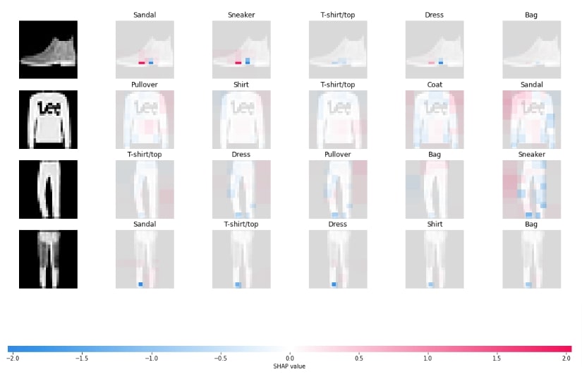
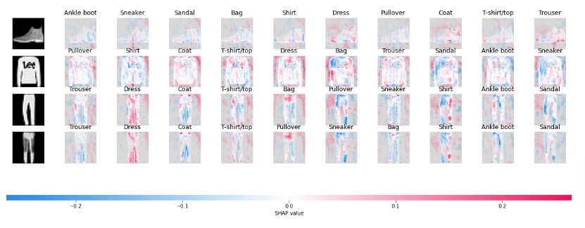
Image Plots¶

Below, we have created an image plot using shap values generated in the previous cell for 4 test images. The shades of red values represent pixels that contributed positively to prediction and shades of blue values represent pixels that contributed negatively to predictions. From the below result, it seems that the masker is not doing that good job. In the next few cells, we have tried different maskers.

shap.image_plot(shap_values)

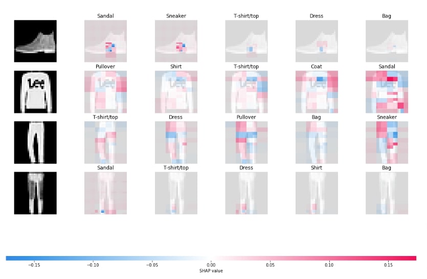
In the below cell, we have created an explainer object again using inpaint_ns masker this time. We generated shap values for the first 4 test images using this new explainer and created an image plot from it. The results look a little better compared to the previous image plot but not that good.

masker = shap.maskers.Image("inpaint_ns", X_train[0].shape)

explainer = shap.Explainer(make_predictions, masker, output_names=class_labels)

shap_values = explainer(X_test[:4].to_py(), outputs=shap.Explanation.argsort.flip[:5])

shap.image_plot(shap_values)

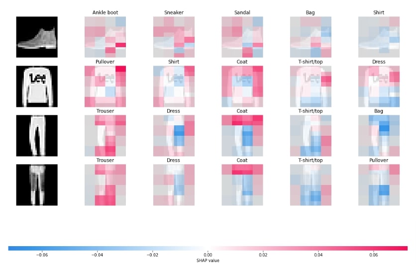
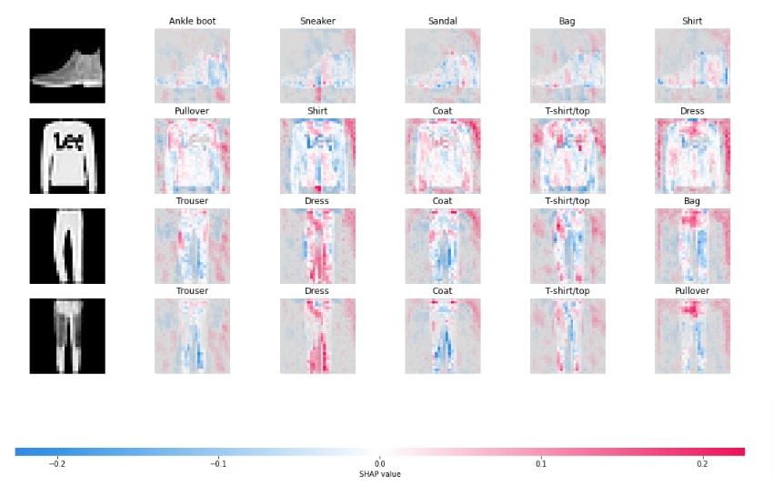
In the below cell, we have created a partition explainer object again using blurr masker. We have provided a tuple of integers specifying the size of the kernel that will be used for blurring. We can notice that the results are better compared to previous maskers.

masker = shap.maskers.Image("blur(28,28)", X_train[0].shape)

explainer = shap.Explainer(make_predictions, masker, output_names=class_labels)

shap_values = explainer(X_test[:4].to_py(), outputs=shap.Explanation.argsort.flip[:5])

shap.image_plot(shap_values)

Visualize SHAP Values For Incorrect Predictions¶

In this section, we have created visualized shap values for wrong predictions. We have first retrieved the indexes of wrong samples by comparing predictions of test samples with actual labels. Then, we have taken 4 test samples for which our model is predicting wrong results. We have printed actual labels, predicted labels, and the probability of prediction by our model for each sample.

wrong_preds_idx = np.argwhere(Y_test!=Y_test_preds)

X_batch = X_test[wrong_preds_idx.flatten()[:4]]
Y_batch = Y_test[wrong_preds_idx.flatten()[:4]]

print("Actual Labels    : {}".format([mapping[i] for i in Y_batch]))
logits_preds = model.apply(final_weights, X_batch)
probs = linen.softmax(logits_preds)
print("Predicted Labels : {}".format([mapping[i] for i in jnp.argmax(probs, axis=1).to_py()]))
print("Probabilities : {}".format(np.max(probs, axis=1)))

Actual Labels    : ['Sneaker', 'Sandal', 'Ankle boot', 'Coat']
Predicted Labels : ['Bag', 'Sneaker', 'Sandal', 'Pullover']
Probabilities : [0.6987277 0.5704662 0.7444548 0.3523756]

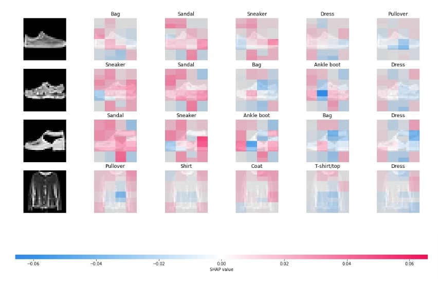
Image Plots¶

Below, we have created an image plot using shap values generated for wrongly predicted images using blurr masker.

masker = shap.maskers.Image("blur(28,28)", X_train[0].shape)

explainer = shap.Explainer(make_predictions, masker, output_names=class_labels)

shap_values = explainer(X_batch.to_py(), outputs=shap.Explanation.argsort.flip[:5])

shap.image_plot(shap_values)

7. Explain Predictions Using Permutation Explainer ¶

In this section, we have explained model predictions using Permutation explainer. The permutation explainer iterates through all permutations of features in forwarding and backward directions to generate shap values. The permutation explainer can be created using PermutationExplainer() constructor by giving the same arguments as that of the partition explainer.

Below, we have created a permutation explainer with blurr masker that we'll use to generate shap values.

masker = shap.maskers.Image("blur(28,28)", X_train[0].shape)

explainer = shap.PermutationExplainer(make_predictions, masker, output_names=class_labels)

explainer

<shap.explainers._permutation.Permutation.__init__.<locals>.Permutation at 0x7f95ec8e1790>

Visualize SHAP Values For Correct Predictions¶

In this section, we have explained images which predicted correctly by our model.

Below, we have generated shap values for our first 4 test images using the permutation explainer created in the previous cell. Then, in the next cell, we have printed actual labels of images, predicted labels, and predicted probabilities.

shap_values = explainer(X_test[:4].to_py(), max_evals=1600, outputs=shap.Explanation.argsort.flip[:5])

shap_values.shape

Permutation explainer: 5it [01:32, 23.04s/it]

(4, 28, 28, 1, 10)

print("Actual Labels    : {}".format([mapping[i] for i in Y_test[:4]]))
logits_preds = model.apply(final_weights, X_test[:4])
probs = linen.softmax(logits_preds)
print("Predicted Labels : {}".format([mapping[i] for i in jnp.argmax(probs, axis=1).to_py()]))
print("Probabilities : {}".format(np.max(probs, axis=1)))

Actual Labels    : ['Ankle boot', 'Pullover', 'Trouser', 'Trouser']
Predicted Labels : ['Ankle boot', 'Pullover', 'Trouser', 'Trouser']
Probabilities : [0.9174614  0.9944201  0.9999931  0.99995995]

Y_preds = model.apply(final_weights, X_test[:4])

Y_preds = Y_preds.argsort()[:, ::-1]
Y_labels = [[class_labels[val] for val in row] for row in Y_preds]
Y_labels = np.array(Y_labels)

Y_labels

array([['Ankle boot', 'Sneaker', 'Sandal', 'Bag', 'Shirt', 'Dress',
        'Pullover', 'Coat', 'T-shirt/top', 'Trouser'],
       ['Pullover', 'Shirt', 'Coat', 'T-shirt/top', 'Dress', 'Bag',
        'Trouser', 'Sandal', 'Ankle boot', 'Sneaker'],
       ['Trouser', 'Dress', 'Coat', 'T-shirt/top', 'Bag', 'Pullover',
        'Sneaker', 'Shirt', 'Ankle boot', 'Sandal'],
       ['Trouser', 'Dress', 'Coat', 'T-shirt/top', 'Pullover', 'Sneaker',
        'Bag', 'Shirt', 'Ankle boot', 'Sandal']], dtype='<U11')

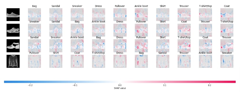
Image Plots¶

In this section, we have plotted shap values using image_plot() for explanation purposes.

shap.image_plot(shap_values, labels=Y_labels)

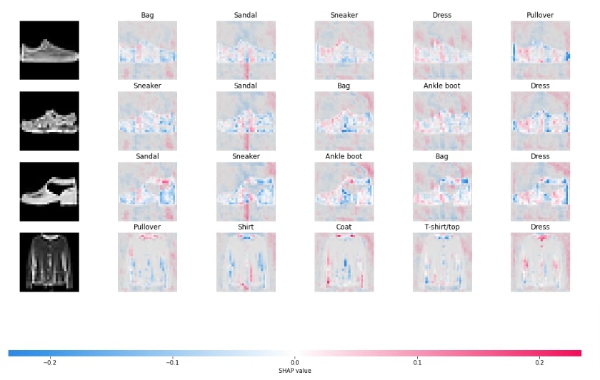
shap.image_plot(shap_values[:,:,:,:,:5], labels=Y_labels[:,:5])

Visualize SHAP Values For Incorrect Predictions¶

In this section, we have generated shap values for wrong predictions using a permutation explainer. The code is almost a repeat of previous sections hence we have not included a detailed explanation.

wrong_preds_idx = np.argwhere(Y_test!=Y_test_preds)

X_batch = X_test[wrong_preds_idx.flatten()[:4]]
Y_batch = Y_test[wrong_preds_idx.flatten()[:4]]

print("Actual Labels    : {}".format([mapping[i] for i in Y_batch]))
logits_preds = model.apply(final_weights, X_batch)
probs = linen.softmax(logits_preds)
print("Predicted Labels : {}".format([mapping[i] for i in jnp.argmax(probs, axis=1).to_py()]))
print("Probabilities : {}".format(np.max(probs, axis=1)))

Actual Labels    : ['Sneaker', 'Sandal', 'Ankle boot', 'Coat']
Predicted Labels : ['Bag', 'Sneaker', 'Sandal', 'Pullover']
Probabilities : [0.6987277 0.5704662 0.7444548 0.3523756]

masker = shap.maskers.Image("blur(28,28)", X_train[0].shape)

explainer = shap.PermutationExplainer(make_predictions, masker, output_names=class_labels)

shap_values = explainer(X_batch.to_py(), max_evals=1600, outputs=shap.Explanation.argsort.flip[:5])

shap_values.shape

Permutation explainer: 5it [01:31, 22.95s/it]

(4, 28, 28, 1, 10)

Y_preds = model.apply(final_weights, X_batch)

Y_preds = Y_preds.argsort()[:, ::-1]
Y_labels = [[class_labels[val] for val in row] for row in Y_preds]
Y_labels = np.array(Y_labels)

Y_labels

array([['Bag', 'Sandal', 'Sneaker', 'Dress', 'Pullover', 'Ankle boot',
        'Shirt', 'Trouser', 'T-shirt/top', 'Coat'],
       ['Sneaker', 'Sandal', 'Bag', 'Ankle boot', 'Dress', 'Pullover',
        'Shirt', 'Coat', 'Trouser', 'T-shirt/top'],
       ['Sandal', 'Sneaker', 'Ankle boot', 'Bag', 'Dress', 'Pullover',
        'Shirt', 'T-shirt/top', 'Coat', 'Trouser'],
       ['Pullover', 'Shirt', 'Coat', 'T-shirt/top', 'Dress', 'Bag',
        'Sandal', 'Trouser', 'Ankle boot', 'Sneaker']], dtype='<U11')

Image Plots¶

shap.image_plot(shap_values, labels=Y_labels)

shap.image_plot(shap_values[:,:,:,:,:5], labels=Y_labels[:,:5])

This ends our small tutorial explaining how we can generate SHAP values for predictions made by an image classification network designed using Flax (JAX). Please feel free to let us know your views in the comments section.

References¶

Sunny Solanki

Comfortable Learning through Video Tutorials?

If you are more comfortable learning through video tutorials then we would recommend that you subscribe to our YouTube channel.

Stuck Somewhere? Need Help with Coding? Have Doubts About the Topic/Code?

When going through coding examples, it's quite common to have doubts and errors.

If you have doubts about some code examples or are stuck somewhere when trying our code, send us an email at coderzcolumn07@gmail.com. We'll help you or point you in the direction where you can find a solution to your problem.

You can even send us a mail if you are trying something new and need guidance regarding coding. We'll try to respond as soon as possible.

Want to Share Your Views? Have Any Suggestions?

If you want to

provide some suggestions on topic
share your views
include some details in tutorial
suggest some new topics on which we should create tutorials/blogs

Please feel free to contact us at coderzcolumn07@gmail.com. We appreciate and value your feedbacks. You can also support us with a small contribution by clicking DONATE.

shap-values, image-classification, Flax, JAX

Sunny Solanki

Software Developer | Youtuber | Bonsai Enthusiast

Subscribe to Our YouTube Channel

Tutorial Categories

Artificial Intelligence (83)
Data Science (84)
Digital Marketing (8)
Machine Learning (38)
Python (131)

Explain Flax (JAX) Image Classification Network Predictions using SHAP Values¶

Important Sections Of Tutorial¶

1. Load Data ¶

2. Define CNN ¶

3. Define Loss ¶

4. Train Network ¶

5. Evaluate Model Performance ¶

6. Explain Predictions Using Partition Explainer ¶

Visualize SHAP Values For Correct Predictions¶

Image Plots¶

Visualize SHAP Values For Incorrect Predictions¶

Image Plots¶

7. Explain Predictions Using Permutation Explainer ¶

Visualize SHAP Values For Correct Predictions¶

Image Plots¶

Visualize SHAP Values For Incorrect Predictions¶

Image Plots¶

References¶

Sunny Solanki

Comfortable Learning through Video Tutorials?

Stuck Somewhere? Need Help with Coding? Have Doubts About the Topic/Code?

Want to Share Your Views? Have Any Suggestions?

Sunny Solanki

Subscribe to Our YouTube Channel

Tutorial Categories

Newsletter Subscription