Flax (JAX): Grad-CAM
Interpreting the results of the deep neural networks has become a quite common practice nowadays in a deep learning community. As the models become deep and complex that are hard to understand, we need to look at which parts of the input data are used by the model to make predictions. This can help us make better decisions and understand whether our model has generalized or not. Whether our model is using the parts of data that it generally makes sense to use for making predictions. Let's say for example in the cat vs dog image classification task, the model should use pixels in an image that contribute to cat or dog in the image and not some background pixels.
As a part of this tutorial, we have explained an algorithm named Grad-CAM (Gradient-weighted Class Activation Mapping) that let us look at parts of an image that contributed to the prediction. The grad-CAM algorithm uses the gradients of any target (say 'cat' in a classification network) flowing into the final convolution layer to produce a coarse localization map highlighting the important regions in the image for predicting the concept. Basically, it highlights activations that contributed most to predicting the particular category using gradients of the last convolution layer with respect to predicted output. The output of the grad-CAM algorithm is a heatmap with the same shape as that of the image which we can overlay over the image to see which parts of the image contributed to the prediction. Below, we have highlighted the steps of the grad-CAM algorithm.
Steps of Grad-CAM
- Capture the output of the last convolution layer of the network.
- Take gradient of last convolution layer with respect to prediction probability. (We can take predictions with respect to any class we want. In our case, we'll take prediction with the highest probability. We can look at other probabilities as well)
- Average gradients calculated in the previous step at axis which has the same dimension as output channels of last convolution layer. The output of this step will be 1D array that has the same numbers as that of output channels of the last convolution layer.
- Multiply convolution layer output with averaged gradients from the previous step at output channel level, i.e. first channel output should be multiplied with first averaged value, second should be multiplied with the second value, and so on.
- Average output from the previous step at channel level to create 2D heatmap that has the same dimension as that of image.
- Normalize heatmap (Optional step but recommended as it helps improve results).
The steps will become more clear when we explain with an example below.
In this tutorial, we have explained step by step guide to implement Grad-CAM algorithm for Flax (JAX) networks. We have trained a simple CNN on Fashion MNIST dataset and then interpreted the predictions using Grad-CAM algorithm.
Below, we have highlighted important sections of tutorial to give an overview of the material covered.
Important Sections Of Tutorial
- Load Data
- Define CNN
- Define Loss
- Train Network
- Evaluate Network Performance
- Grad-CAM With Respect To Last Convolution Layer (Step By Step)
- Grad-CAM With Respect To Second Last Convolution Layer
- Grad-CAM With Respect To First Convolution Layer
Below, we have imported the necessary libraries and printed the versions that we have used in our tutorial.
import jax

print("JAX Version : {}".format(jax.__version__))
import flax

print("FLAX Version : {}".format(flax.__version__))
import optax

print("OPTAX Version : {}".format(optax.__version__))
1. Load Data 
In this section, we have loaded the Fashion MNIST dataset available from keras. The dataset has grayscale images of shape (28,28) for 10 different fashion items. The dataset is already divided into the train (60k images) and test (10k images) sets. After loading datasets, we have converted them to JAX arrays as required by networks. Below, we have included mapping from the target class index to target class names for reference purposes.
| Label | Description |
|---|---|
| 0 | T-shirt/top |
| 1 | Trouser |
| 2 | Pullover |
| 3 | Dress |
| 4 | Coat |
| 5 | Sandal |
| 6 | Shirt |
| 7 | Sneaker |
| 8 | Bag |
| 9 | Ankle boot |
from tensorflow import keras
from sklearn.model_selection import train_test_split
from jax import numpy as jnp
import numpy as np

(X_train, Y_train), (X_test, Y_test) = keras.datasets.fashion_mnist.load_data()

X_train, X_test = X_train.reshape(-1,28,28,1), X_test.reshape(-1,28,28,1)

X_train, X_test = jnp.array(X_train), jnp.array(X_test)

X_train, X_test = X_train/255.0, X_test/255.0

classes =  np.unique(Y_train)
class_labels = ["T-shirt/top","Trouser","Pullover","Dress","Coat","Sandal","Shirt","Sneaker","Bag","Ankle boot"]
mapping = dict(zip(classes, class_labels))

X_train.shape, X_test.shape, Y_train.shape, Y_test.shape
2. Define CNN 
In this section, we have defined a simple convolutional neural network that we'll use to classify our grayscale images. The network has 3 convolution layers and one dense layer. The convolution layers have output channels of sizes 48, 32, and 16 respectively. The relu activation function is applied to the output of each convolution layer. The output of the last convolution layer is flattened after applying relu and fed into a dense layer. The dense layer has 10 output units which are the same as a number of target classes.
Please make a NOTE that we have not covered a detailed description of network creation using Flax as we have already covered it in the below tutorials. Please feel free to check them if you don't have a background on Flax.
from flax import linen
from jax import random

class CNN(linen.Module):
    def setup(self):
        self.conv1 = linen.Conv(features=48, kernel_size=(3,3), padding="SAME", name="CONV1")
        self.conv2 = linen.Conv(features=32, kernel_size=(3,3), padding="SAME", name="CONV2")
        self.conv3 = linen.Conv(features=16, kernel_size=(3,3), padding="SAME", name="CONV3")
        self.linear1 = linen.Dense(len(classes), name="DENSE")

    def __call__(self, inputs):
        x = linen.relu(self.conv1(inputs))
        x = linen.relu(self.conv2(x))
        x = linen.relu(self.conv3(x))

        x = x.reshape((x.shape[0], -1))
        logits = self.linear1(x)

        return logits #linen.softmax(x)
seed = jax.random.PRNGKey(0)

model = CNN()
params = model.init(seed, X_train[:5])

for layer_params in params["params"].items():
    print("Layer Name : {}".format(layer_params[0]))
    weights, biases = layer_params[1]["kernel"], layer_params[1]["bias"]
    print("\tLayer Weights : {}, Biases : {}".format(weights.shape, biases.shape))
preds = model.apply(params, X_train[:5])

preds.shape
3. Define Loss 
In this section, we have defined a loss function for our image classification task. We'll be using cross entropy loss for our purpose. The function takes network parameters, input samples, and actual target values of those samples as input. It then performs a forward pass through the network to make predictions and one hot encodes actual target values. Then, it calculates loss using softmax_cross_entropy() function available from Optax python library.
def CrossEntropyLoss(weights, input_data, actual):
    logits = model.apply(weights, input_data)
    one_hot_actual = jax.nn.one_hot(actual, num_classes=len(classes))
    return optax.softmax_cross_entropy(logits, one_hot_actual).sum()
4. Train Network 
In this section, we have trained our CNN on the fashion MNIST dataset. Below, we have first defined a function that will perform the whole training process. The function takes training data (X, Y), validation data (X_val, Y_val), number of epochs, network parameters, optimizer state, and batch size as input. The function executes the training loop number of epoch times and returns updated network parameters at the end. During each epoch, it loops through training data in batches. For each batch of data, it calculates predictions, calculates loss value, calculates gradients, and updates network weights using gradients. It also keeps track of loss value for each batch and prints average loss at the end of one training epoch. The function also calculates validation accuracy at the end of the epoch and prints it.
from jax import value_and_grad
from tqdm import tqdm
from sklearn.metrics import accuracy_score

def TrainModelInBatches(X, Y, X_val, Y_val, epochs, weights, optimizer_state, batch_size=32):
    for i in range(1, epochs+1):
        batches = jnp.arange((X.shape[0]//batch_size)+1) ### Batch Indices

        losses = [] ## Record loss of each batch
        for batch in tqdm(batches):
            if batch != batches[-1]:
                start, end = int(batch*batch_size), int(batch*batch_size+batch_size)
            else:
                start, end = int(batch*batch_size), None

            X_batch, Y_batch = X[start:end], Y[start:end] ## Single batch of data

            loss, gradients = value_and_grad(CrossEntropyLoss)(weights, X_batch,Y_batch)

            ## Update Weights
            updates, optimizer_state = optimizer.update(gradients, optimizer_state)
            weights = optax.apply_updates(weights, updates)

            losses.append(loss) ## Record Loss

        print("CrossEntropyLoss : {:.3f}".format(jnp.array(losses).mean()))

        Y_val_preds = model.apply(weights, X_val)
        val_acc = accuracy_score(Y_val, jnp.argmax(Y_val_preds, axis=1))
        print("Validation  Accuracy : {:.3f}".format(val_acc))

    return weights
Below, we are actually training our network using a function defined in the previous cell by initializing necessary parameters. We have initialized batch size to 256, epochs to 8, and learning rate to 0.001. Then, we have initialized the network, network parameters, and Adam optimizer. At last, we have called our training routine with the necessary parameters to perform training. We can notice from the loss and validation accuracy getting printed after each epoch that our model is doing a good job.
seed = random.PRNGKey(0)
batch_size=256
epochs=8
learning_rate = jnp.array(1e-3)

model = CNN()
weights = model.init(seed, X_train[:5])

optimizer = optax.adam(learning_rate=learning_rate) ## Initialize Adam Optimizer
optimizer_state = optimizer.init(weights)

final_weights = TrainModelInBatches(X_train, Y_train, X_test, Y_test, epochs, weights, optimizer_state, batch_size=batch_size)
5. Evaluate Network Performance 
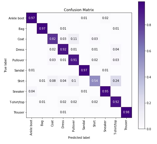
In this section, we have evaluated the network performance by calculating accuracy, confusion matrix and classification report metrics on test predictions. We can notice from the metrics results that our model is doing an almost good job in predicting each target category.
Below, we have calculated all metrics using functions available from scikit-learn. Please feel free to check the below link if you want to learn about various ML metrics available through sklearn.
In the next cell after the below cell, we have plotted the confusion matrix. We can notice from the results that our model is not doing that good job at predicting category Shirt and confusing it very often with category T-shirt/top. This makes sense as images of both categories look almost the same but still, we can try different models to improve better accuracy.
Please feel free to check the below tutorial if you want to learn about scikit-plot.
from sklearn.metrics import accuracy_score, confusion_matrix, classification_report

Y_test_preds = model.apply(final_weights, X_test)
Y_test_preds = jnp.argmax(Y_test_preds, axis=1)

print("Test Accuracy : {}".format(accuracy_score(Y_test, Y_test_preds)))
print("\nConfusion Matrix : ")
print(confusion_matrix(Y_test, Y_test_preds))
print("\nClassification Report :")
print(classification_report(Y_test, Y_test_preds, target_names=class_labels))
from sklearn.metrics import confusion_matrix
import scikitplot as skplt
import matplotlib.pyplot as plt

skplt.metrics.plot_confusion_matrix([class_labels[i] for i in Y_test], [class_labels[i] for i in Y_test_preds],
                                    normalize=True,
                                    title="Confusion Matrix",
                                    cmap="Purples",
                                    hide_zeros=True,
                                    figsize=(8,8)
                                    );
plt.xticks(rotation=90);
6. Grad-CAM With Respect To Last Convolution Layer (Step By Step) 
In this section, we have explained a step-by-step guide to implement Grad-CAM algorithm using Flax (JAX). We have implemented Grad-CAM in this section with respect to the last convolution layer. The reason behind this is that the last layer has final combined patterns of previous layers which are then fed to dense layers before making decisions. All other convolution layers also learn different patterns and we'll look at them in the next sections.
1. Capture Output Of Last Convolution Layer
In this section, we are capturing the output of the last convolution layer. In order to do that we have created another network that has the same first 3 convolution layers as our original network. The forward pass through the network returns the output of the third convolution layer.
After defining the network, we have randomly selected one sample from data and performed a forward pass through this new network to capture the output of the last convolution layer. In order to perform forward pass, we have used network parameters which are trained network parameters of our original network. We can notice from the result that the output shape of our convolution layer is (1,28,28,16) where 16 represents output channels and batch size of 1 represents a single sample.
from flax import linen
from jax import random

class ModifiedCNN1(linen.Module):
    def setup(self):
        self.conv1 = linen.Conv(features=48, kernel_size=(3,3), padding="SAME", name="CONV1")
        self.conv2 = linen.Conv(features=32, kernel_size=(3,3), padding="SAME", name="CONV2")
        self.conv3 = linen.Conv(features=16, kernel_size=(3,3), padding="SAME", name="CONV3")

    def __call__(self, inputs):
        x = linen.relu(self.conv1(inputs))
        x = linen.relu(self.conv2(x))
        x = linen.relu(self.conv3(x))
        return x
import random

modified_cnn1 = ModifiedCNN1()

idx = random.randint(0, len(X_test)) ## Randomly Select Sample

conv_output = modified_cnn1.apply(final_weights, X_test[idx:idx+1]) ## Perform forward pass to get output of last conv layer.

conv_output.shape
2. Calculate Gradients Of Prediction With Respect To Output Of Last Conv Layer
In this section, we have calculated the gradient of the last convolution layer output with respect to maximum prediction probability. In order to perform this step, we have designed another simple network that takes the last convolution layer output as input and returns network prediction after applying a linear layer to it as in our original network. In short, here, we are performing the remaining half of our network forward pass. The network returns 10 probabilities per sample.
After defining the network, we have defined a function that takes as input convolution layer input and returns maximum probability by performing forward pass through below network. To perform forward pass, it uses trained network parameters that we had from the training of our network earlier.
Now, to calculate gradients, we have used grad() function from JAX and wrapped our function inside it. This returns another function that calculates the gradient of the input value to the function with respect to the output of the function. In our case, this will calculate the gradient of convolution layer output with respect to maximum probability.
After calculating the gradient of convolution layer output with respect to maximum probability, we have also printed its shape which (1,28,28,16) same as the convolution layer output shape.
Please make a NOTE that we have calculated gradient with respect to maximum probability which will be predicted class. We can compute gradient with respect to some other probability as well if we want to check activations for some other class than the one predicted by the network using maximum probability.
from flax import linen
from jax import random

class ModifiedCNN2(linen.Module):
    def setup(self):
        self.linear1 = linen.Dense(len(classes), name="DENSE")

    def __call__(self, inputs):
        x = inputs.reshape((inputs.shape[0], -1))
        logits = self.linear1(x)

        return linen.softmax(logits)
def GradCAM(conv_output):
    modified_cnn2 = ModifiedCNN2()
    preds = modified_cnn2.apply(final_weights, conv_output)
    return preds.max()
from jax import grad

grad_GradCAM = grad(GradCAM)

grads = grad_GradCAM(conv_output)

grads.shape
modified_cnn2 = ModifiedCNN2()
preds = modified_cnn2.apply(final_weights, conv_output)

print("Actual    Category : {}".format(mapping[Y_test[idx]]))
print("Predicted Category : {}".format(mapping[preds.argmax(axis=-1).to_py()[0]]))
3. Average Gradients
In this section, we have averaged gradients in a way that after averaging we have values that are the same as the output channels of the last convolution layer. In our case the shape of gradients is (1,28,28,16), hence we have first squeezed it to remove extra dimension from the beginning (new shape (28,28,16)) and averaged at 0th & 1st axis to get 16 values as output which is same as the last convolution layer output channels.
pooled_grads = grads.squeeze().mean((0,1))

pooled_grads
4. Multiply Pooled Gradients With Conv Layer Output
In this section, we have multiplied the output of the convolution layer with averaged gradients from the previous step at channel levels. This way output of each convolution layer output channel will be multiplied with the average gradient value of that channel.
conv_output = conv_output.squeeze()

conv_output.shape
for i in range(len(pooled_grads)):
    conv_output = conv_output.at[:,:,i].set(conv_output[:,:,i] * pooled_grads[i])
5. Average Output To Create Heatmap And Normalize Heatmap
This is the last step in our algorithm where we have calculated the average of output from the previous step at the channel level. This way the output will be of shape (28,28) which is the same as the shape of our image and we'll call it heatmap. This heatmap can be visualized and compared with the original image to look at activations that contributed to the prediction of a particular category. We also generally normalize the heatmap for better results.
heatmap = conv_output.mean(axis=-1)

#heatmap = linen.relu(heatmap) / heatmap.max()
#heatmap = heatmap / heatmap.max()
heatmap = (heatmap - heatmap.min()) / (heatmap.max() - heatmap.min())


heatmap.shape
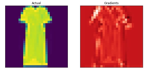
6. Visualize Actual Image And Heatmap
In this section, we have visualized the original image and heatmap next to each other to compare and look at activations contributing to prediction.
import matplotlib
import matplotlib.pyplot as plt

def plot_actual_and_heatmap(idx, heatmap):
    cmap = matplotlib.cm.get_cmap("Reds")

    fig = plt.figure(figsize=(10,10))
    ax1 = fig.add_subplot(121)
    ax1.imshow(X_test[idx].to_py().squeeze());
    ax1.set_title("Actual");
    ax1.set_xticks([],[]);ax1.set_yticks([],[]);

    ax2 = fig.add_subplot(122)
    ax2.imshow(heatmap, cmap="Reds");
    ax2.set_title("Gradients");
    ax2.set_xticks([],[]);ax2.set_yticks([],[]);

plot_actual_and_heatmap(idx, heatmap.to_py())
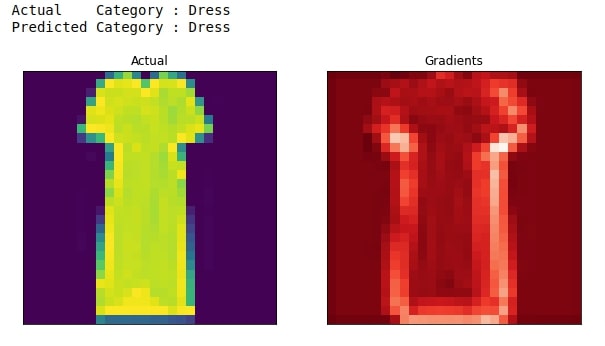
7. Grad-CAM With Respect To Second Last Convolution Layer 
In this section, we have performed the Grad-CAM algorithm with respect to the output of the second last convolution layer. We have followed almost the same steps as we explained in the previous section. The major difference is in how we created two networks. We generally split our original network at the layer where we want to perform Grad-CAM algorithm.
from flax import linen
from jax import random

## Capture Output Of Convolution Layer
class ModifiedCNN1(linen.Module):
    def setup(self):
        self.conv1 = linen.Conv(features=48, kernel_size=(3,3), padding="SAME", name="CONV1")
        self.conv2 = linen.Conv(features=32, kernel_size=(3,3), padding="SAME", name="CONV2")

    def __call__(self, inputs):
        x = linen.relu(self.conv1(inputs))
        x = linen.relu(self.conv2(x))
        return x

modified_cnn1 = ModifiedCNN1()
conv_output = modified_cnn1.apply(final_weights, X_test[idx:idx+1])

## Calculate Gradients Of Prediction With Respect To Output Of Last Conv Layer
class ModifiedCNN2(linen.Module):
    def setup(self):
        self.conv3 = linen.Conv(features=16, kernel_size=(3,3), padding="SAME", name="CONV3")
        self.linear1 = linen.Dense(len(classes), name="DENSE")

    def __call__(self, inputs):
        x = linen.relu(self.conv3(inputs))
        x = x.reshape((x.shape[0], -1))
        logits = self.linear1(x)
        return linen.softmax(logits)

def GradCAM(conv_output):
    modified_cnn2 = ModifiedCNN2()
    preds = modified_cnn2.apply(final_weights, conv_output)
    return preds.max()

grad_GradCAM = grad(GradCAM)
grads = grad_GradCAM(conv_output)

modified_cnn2 = ModifiedCNN2()
preds = modified_cnn2.apply(final_weights, conv_output)

print("Actual    Category : {}".format(mapping[Y_test[idx]]))
print("Predicted Category : {}".format(mapping[preds.argmax(axis=-1).to_py()[0]]))

## Average Gradients
pooled_grads = grads.squeeze().mean((0,1))

## Multiply Pooled Gradients With Conv Layer Output
conv_output = conv_output.squeeze()

for i in range(len(pooled_grads)):
    conv_output = conv_output.at[:,:,i].set(conv_output[:,:,i] * pooled_grads[i])

## Average Output To Create Heatmap And Normalize Heatmap
heatmap = conv_output.mean(axis=-1)
#heatmap = linen.relu(heatmap) / heatmap.max()
#heatmap = heatmap / heatmap.max()
heatmap = (heatmap - heatmap.min()) / (heatmap.max() - heatmap.min())

## Visualize Results
plot_actual_and_heatmap(idx, heatmap.to_py())
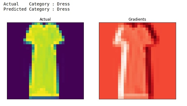
8. Grad-CAM With Respect To First Convolution Layer 
In this section, we have performed Grad-CAM with respect to the third last layer which is actually the first layer of our network.
from flax import linen
from jax import random

## Capture Output Of Convolution Layer
class ModifiedCNN1(linen.Module):
    def setup(self):
        self.conv1 = linen.Conv(features=48, kernel_size=(3,3), padding="SAME", name="CONV1")

    def __call__(self, inputs):
        x = linen.relu(self.conv1(inputs))
        return x

modified_cnn1 = ModifiedCNN1()
conv_output = modified_cnn1.apply(final_weights, X_test[idx:idx+1])

## Calculate Gradients Of Prediction With Respect To Output Of Last Conv Layer
class ModifiedCNN2(linen.Module):
    def setup(self):
        self.conv2 = linen.Conv(features=32, kernel_size=(3,3), padding="SAME", name="CONV2")
        self.conv3 = linen.Conv(features=16, kernel_size=(3,3), padding="SAME", name="CONV3")
        self.linear1 = linen.Dense(len(classes), name="DENSE")

    def __call__(self, inputs):
        x = linen.relu(self.conv2(inputs))
        x = linen.relu(self.conv3(x))
        x = x.reshape((x.shape[0], -1))
        logits = self.linear1(x)
        return linen.softmax(logits)

def GradCAM(conv_output):
    modified_cnn2 = ModifiedCNN2()
    preds = modified_cnn2.apply(final_weights, conv_output)
    return preds.max()

grad_GradCAM = grad(GradCAM)
grads = grad_GradCAM(conv_output)

modified_cnn2 = ModifiedCNN2()
preds = modified_cnn2.apply(final_weights, conv_output)

print("Actual    Category : {}".format(mapping[Y_test[idx]]))
print("Predicted Category : {}".format(mapping[preds.argmax(axis=-1).to_py()[0]]))

## Average Gradients
pooled_grads = grads.squeeze().mean((0,1))

## Multiply Pooled Gradients With Conv Layer Output
conv_output = conv_output.squeeze()

for i in range(len(pooled_grads)):
    conv_output = conv_output.at[:,:,i].set(conv_output[:,:,i] * pooled_grads[i])

## Average Output To Create Heatmap And Normalize Heatmap
heatmap = conv_output.mean(axis=-1)
#heatmap = linen.relu(heatmap) / heatmap.max()
#heatmap = heatmap / heatmap.max()
heatmap = (heatmap - heatmap.min()) / (heatmap.max() - heatmap.min())

## Visualize Results
plot_actual_and_heatmap(idx, heatmap.to_py())
This ends our small tutorial explaining how we can perform Grad-CAM algorithm with Flax (JAX) image classification networks. Please feel free to let us know your views in the comments section.
References
 Sunny Solanki
Sunny Solanki
Intro: Software Developer | Youtuber | Bonsai Enthusiast
About: Sunny Solanki holds a bachelor's degree in Information Technology (2006-2010) from L.D. College of Engineering. Post completion of his graduation, he has 8.5+ years of experience (2011-2019) in the IT Industry (TCS). His IT experience involves working on Python & Java Projects with US/Canada banking clients. Since 2020, he’s primarily concentrating on growing CoderzColumn.
His main areas of interest are AI, Machine Learning, Data Visualization, and Concurrent Programming. He has good hands-on with Python and its ecosystem libraries.
Apart from his tech life, he prefers reading biographies and autobiographies. And yes, he spends his leisure time taking care of his plants and a few pre-Bonsai trees.
Contact: sunny.2309@yahoo.in


![YouTube Subscribe]() Comfortable Learning through Video Tutorials?
Comfortable Learning through Video Tutorials?
If you are more comfortable learning through video tutorials then we would recommend that you subscribe to our YouTube channel.
![Need Help]() Stuck Somewhere? Need Help with Coding? Have Doubts About the Topic/Code?
Stuck Somewhere? Need Help with Coding? Have Doubts About the Topic/Code?
 Stuck Somewhere? Need Help with Coding? Have Doubts About the Topic/Code?
When going through coding examples, it's quite common to have doubts and errors.
If you have doubts about some code examples or are stuck somewhere when trying our code, send us an email at coderzcolumn07@gmail.com. We'll help you or point you in the direction where you can find a solution to your problem.
You can even send us a mail if you are trying something new and need guidance regarding coding. We'll try to respond as soon as possible.
![Share Views]() Want to Share Your Views? Have Any Suggestions?
Want to Share Your Views? Have Any Suggestions?
 Want to Share Your Views? Have Any Suggestions?
If you want to
- provide some suggestions on topic
- share your views
- include some details in tutorial
- suggest some new topics on which we should create tutorials/blogs
 flax, jax, grad-cam, image-classification