Convolutional Neural Networks (CNN or ConvNet)¶

The convolutional neural network is a type of artificial neural network which has proven giving very good results for visual imagery over the last few years. Over the years many version of convolutional neural network has been designed to solve many tasks as well as to win image net competitions. Any artificial neural network which uses the convolution layer in its architecture can be considered as ConvNet. ConvNets typically start with recognizing smaller patterns/objects in data and later on combines these patterns/objects further using more convolution layers to predict the whole object. Yann Lecun developed the first successful ConvNet by applying backpropagation to it during the 1990s called LeNet. Later on, different versions of ConvNet has won imagenet competitions a few times. We'll be discussing convolutional neural net workings as well as it's applications in this article.

We'll start by explaining mathematical operation convolution.

What Is Convolution?¶

From a computer science point of view convolution operation refers to the application of one small array(commonly refers to as a filter) on another big array in some way to produce third output array. We multiply filter array with part(same size as filter array) of the original big array starting from the top and then sum up all values of resulting array to produce first value of the final array. We then keep on moving by one step to the next value of the big array and repeat the same process until the whole big array is processed from left to right. Please make a note that the convolution operation decreases the size of the original array based on filter size. We'll try to explain the whole process with a few examples below to clear understanding further.

Let's define a simple array of size 10 where the first five elements are 0s and the last five elements are 1s.

Let's define a simple filter array of size 3 with all elements as 1/3.

Above filter_arr started multiplying original_arr from starting by moving one step at a time. It then sums up multiplication results to generate the first element of the result. It then repeats the same process till the end of an array is reached.

Note Please make a note that default mode of application with np.convolve is full which appends 0s on both start and end so that all elements of array are processed. There are other modes as well like same which returns resulting array as the same length of original array by adding 0s at end of an original array during convolution operation. We have used mode valid which does not perform any kind of padding of 0s.

Please make a note that above result appends 2 0s at beginning of original array and 2 0s at end of original array.

Please make a note that above result appends one 0 at beginning of original array and one 0 at end of original array.

We can also use ndimage module of scipy to compute convolution which has some more mode available for testing purpose.

From the above result, we can see that it has the same length as the original array but the last element is not 0.666667. The default mode with the convolve function of the ndimage module is reflect which extends the original array with the same last element. Hence our original array had the last element as 1 it got appended at last to get the same size as the original array.

Let's try convolution operation on 2D array.

Let's try to visualize original array.

As we can see above the original filter seems to smooth edge which separates black from white. Filters can perform many things like the above one. As a part of the convolutional neural network, the model learns this filter by training on data to learn intricate patterns.

Please make a note that np.convolve can only work on 1D array. For 2 or more dimensions, we need to use scipy.ndimage convolve function.

We'll now try to understand the architecture of convolution as we have a clear understanding of what is convolution operation.

What Is Called Convolutional Neural Network (Architectural Overview)¶

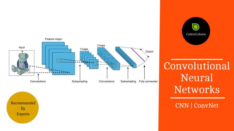
Any artificial neural network which uses convolution layers in its architecture is called a convolutional neural network. Convolutional Neural Network generally performs quite well for image classification/object detection hence we'll try to explain it's architecture from the image classification task point of view. Below we have shown sample CNN architecture for processing images.

Color images are maintained as a three-dimensional array (width x height x channels). Hence CNN neurons of convolution layers are also arranged in a way that applies a list of filters on these 3-dimensional images.

Generally, the architecture of CNN consists of a list of blocks of (Convolution, Pooling) layers followed by fully connected layers. Conv block can consist of a single Convolution layer followed by single pooling layers or even more than one convolution layer followed by a single pooling layer.

Sample Architectures:

$INPUT->CONV->POOL->CONV->POOL->...->FC->OUPUT$

$INPUT->CONV->CONV->POOL->CONV->CONV->POOL->...->FC->OUPUT$

Below are described common layers of CNN:

• Inputs to CNN are generally images of 3 dimensions for RGB images and 2 dimensions for grayscale images.
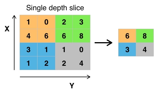
• CONV Layer: It applies convolution operation as described above followed by activation which is generally RELU (Rectified Linear Unit)). It takes as input the number of filters which we discussed above that will be initially initialized randomly or zeros but will get values during training. These filters are weights of convolution layers.

• POOLING Layer: We then apply the pooling layer which reduces the size of activated output from the Conv layer resulting in downsampling. Pooling reduces size in both dimensions for images. Pooling layers do not have any weights to train as it just decreases the size of the input. Below sample image depicts how pooling works.

• Fully Connected Layer: Output of last Pooling layer is flattened converting it to one dimensional and then given as input to fully connected layer. It's then followed by activation function which is generally sigmoid/softmax for classification tasks to predict object.

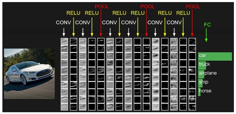
The below image displays how image is transformed when it passes through various layers of CNN.

We can see from the above image that convolution layers followed by pooling layers create a simple representation of an original image to classify it. All deep learning libraries like Keras, Pytorch, Tensorflow, etc provides layers ready-made for convolution and pooling operations. Keras provides a very easy API to design CNNs.Keras, Pytorch, Tensorflow also provide a few famous CNN architecture along with their weights which can be used for transfer learning for other almost same tasks.

We'll now list-down a few common applications of CNN.

Applications of CNN¶

• Object Detection/Image Classification
• Recommendation System
• Object detection in videos
• CNN’s can be used in natural language processing as well for classification
• Time Series Predictions

Pros of CNN¶

• fewer model parameters to train compared to multilayer perceptron.
• Less time required for training due to fewer parameters. (With GPU)
• High Accuracy for image classification problems.
• Once trained same CNN can be used with slightly different tasks with different data using transfer learning

Cons of CNN¶

• Requires a large amount of data to get high accuracy
• Suffers from overfitting if the amount of data is less.
• High Computational Cost(Without GPU)
• CNN suffers from the problem of finding a solution with local optima. Hence they need initial parameter tunning to get global optima.

Famous CNN Architectures¶

Below we have listed some famous CNN architectures. Libraries like Keras, Pytorch, Tensorflow, etc provide these architectures as well as their trained weights which can be used for other image classification tasks.

• LeNet: It was the first successful application of CNN by Yann Lecun. He used it to recognize handwritten zip code digits.
• AlexNet: It was CNN designed by Alex Krizhevsky, Ilya Sutskever, and Geoff Hinton which won Imagenet competition of 2012. This first use of CNN to win imagenet competition popularized CNN considerably. It was the same in concept as that of LeNet but quite deeper and with more than one convolution layers stacked on each other.
• GoogleNet : It was CNN from google team which won Imagenet competition of 2014. The main concept as part of this architecture was inception block which reduced the number of network parameters to train. It also uses average pooling on top of the convolution layer instead of fully connected layers which resulted in a reduction of a number of trainable parameters.
• VGGNet: It was CNN architecture designed by VGG department of Oxford University which was first runner up of 2014 imagenet competition. It’s taken into consideration because it's architecture was quite small compared to other deep complicated architectures in competition.
• ResNet: Residual Network was CNN developed by Kaiming He who won the imagenet competition of 2015. The idea behind ResNet was introducing “identity shortcut connection” that skips one or more layers also refers to as skip connections. ResNets are still quite useful in various image classification tasks.

References¶

The below articles were referred to while creating this article and images were taken from below materials for explanation purpose. Readers can further go through the below articles to enhance their knowledge to the next level.

• Convolutional Neural Network Wikipedia
• CNN guide from stanford
• Gradient-Based Learning Applied to Document Recognition- LeNet
• Object Recognition With Gradient-Based Learning