Transfer Learning using PyTorch (Image Classification)
Transfer learning is a process where a person takes a neural model trained on a large amount of data for some task and uses that pre-trained model for some other task which has somewhat similar data than the training model again from scratch.
It generally refers to the transfer of knowledge from one model to another model which has somewhat similar requirements so that we can reuse weights of the model. We can use such an approach when we don't have enough data or resources to train the model.
Types of transfer learnings:
- convnet as a fixed feature extractor: Here we replace the last fully connected layer of pre-trained network like VGG and replace with layer according to requirement and train only that layer of network keeping all previous layers freeze. Here we
reuse almost whole architectureof VGG except the last few fully connected layers. - finetuning convnet: Here we replace the last fully connected layer of pre-trained network like VGG and then train the whole network slightly for
few epochs on lower learning rateto finetune model according to a new requirement. We also train conv layers here to finetune them for new requirements. We can keep a few earlier layers of conv net fixed and train the last few conv layers or we can train all conv layers. Earlier conv layers have basic shape details like line, circle, etc. Here wereuse almost whole architectureof VGG like conv models. - pre-trained models: Here we take weights released by convolution layers trained large amount of data like imagenet and use these weights in our conv model. Here we
don't reuse architecturebut only use weights of conv layers of VGG like models into our model's layers.
How to decide when we can do transfer learning?
There are various factors when we can decide on transfer learning and level of transfer learning to apply:
- New dataset is similar to an original dataset but small - convnet as fixed future extractor.
- New dataset is similar to original but large - finetuning convnet. Train whole net little bit on low learning rate.
- New dataset is different from original but small - convnet as fixed future extractor.
- New dataset is different from original but large - Design your own conv net and train it but better to initialize it's conv layer weights with weights from some existing well-performing model.
#!pip install --upgrade pip
#!pip install torch torchvision
Importing all necessary libraries
import torch
import torch.nn as nn
import torch.nn.functional as F
import torch.optim as optim
import torchvision
from torchvision import datasets, transforms, models

import matplotlib.pyplot as plt
import numpy as np

import os
import shutil
import glob

print(torch.__version__)
device  = 'cuda' if torch.cuda.is_available() else 'cpu'
print('Cuda available : '+ str((device == 'cuda')))
Downloading Dataset and Extracting
We'll be using the Dog Breeds image dataset provided by Stanford for our purpose. It has around 20k+ images of 120 categories of different dog breeds.
We'll download and unzip it in the current directory.
%%time
!wget http://vision.stanford.edu/aditya86/ImageNetDogs/images.tar
!tar -xf images.tar
#!cp -r Images dogs
!rm images.tar
%ls
Convnet as fixed feature extractor example
We'll be first trying convnet as fixed future extractor where we'll modify the last Linear Layer to output 120 probabilities for each image. We'll also set all layers of the network as non-trainable except the last layer. We'll then train the network by setting different learning rates for few epochs to make it predict the correct output for our purpose.
Creating subdirectories and copying data
We have below designed function which creates a new destination directory and then creates train, val and test subdirectories inside it.
We'll then move 80% of images according to the category to train subfolder, 10% to val subfolder and 10% to test subfolder.
Note: Please make a not that train, val, and test subfolders will have the same structure(dog category subfolders) as original source folder except that number of images inside dog category subfolders will be according to proportion mentioned in the previous sentence.
%%time

def create_ml_file_strcuture_and_move_files(src, dest):
    os.makedirs(os.path.join(dest,'train'), exist_ok=True)
    os.makedirs(os.path.join(dest,'val'), exist_ok=True)
    os.makedirs(os.path.join(dest,'test'), exist_ok=True)

    for directory in os.listdir(src):
        os.makedirs(os.path.join(dest,'train',directory), exist_ok=True)
        os.makedirs(os.path.join(dest,'val',directory), exist_ok=True)
        os.makedirs(os.path.join(dest,'test',directory), exist_ok=True)
        init_path = os.path.join(src, directory)
        all_files = os.listdir(init_path)
        n = len(all_files)
        for file in all_files[:int(0.8*n)]:
            shutil.copy(os.path.join(src,directory,file),os.path.join(dest,'train',directory))
        for file in all_files[int(0.8*n):int(0.9*n)]:
            shutil.copy(os.path.join(src,directory,file),os.path.join(dest,'val',directory))
        for file in all_files[int(0.9*n):]:
            shutil.copy(os.path.join(src,directory,file),os.path.join(dest,'test',directory))

create_ml_file_strcuture_and_move_files('Images','dogs')
Below we are printing count for different folder's images to verify that our original image count does match with train,val, test subfolders images count.
We also verify that all folder structure is properly created.
print('List of subdirs in Images folder : %d'%len(os.listdir('Images')))
print('List of subdirs in dogs/train folder : %d'%len(os.listdir('dogs/train')))
print('List of subdirs in dogs/val folder : %d'%len(os.listdir('dogs/val')))
print('List of subdirs in dogs/test folder : %d'%len(os.listdir('dogs/test')))
print('List of JPGs in original Images directory : %d'%len(glob.glob('Images/*/*.jpg')))
print('List of JPGs in dogs sub directories : %d'%len(glob.glob('dogs/*/*/*.jpg')))
Initializing DataLoaders
Pytorch provides different modules for doing image manipulation in batches named torchvision.
torchvision provides default data loaders which we can use for loading images from folders and transformers which can do various transformations on images like resizing, cropping, converting to tensors, etc.
We'll be loading images from folders using ImageFolder dataset creator and apply 4 transformations to all images. We'll resize them to 256x256 size images, crop center 224x224 pixel image from it, convert image to PyTorch tensor and then do normalization (subtracting mean and dividing by standard deviation).
We need to resize images to 224x224 and do normalization because that is a requirement of the VGG neural network which we'll be using for our purpose. It's setting based on which it performs well.
Also, make a note that we are shuffling images of training and validation data but not of test data. num_workers refers to number parallel threads to run to handle the task.
data_transform = transforms.Compose([
                                        transforms.Resize(256),
                                        transforms.CenterCrop(224),
                                        transforms.ToTensor(),
                                        transforms.Normalize([0.485, 0.456, 0.406], [0.229, 0.224, 0.225])
                                    ])
dsets = {}
dsets['train'] = datasets.ImageFolder('dogs/train', transform=data_transform)
dsets['val'] = datasets.ImageFolder('dogs/val', transform=data_transform)
dsets['test'] = datasets.ImageFolder('dogs/test', transform=data_transform)
loaders = {}
loaders['train'] = torch.utils.data.DataLoader(dsets['train'], batch_size=8, shuffle=True,num_workers=4)
loaders['val'] = torch.utils.data.DataLoader(dsets['val'], batch_size=8, shuffle=True,num_workers=4)
loaders['test'] = torch.utils.data.DataLoader(dsets['test'], batch_size=1, shuffle=False,num_workers=4)
Below we have defined a few lists and dictionaries which we'll be using for a few mappings purpose. By default, we'll get an index of dog which has the highest probability of 120 dog breeds. We'll need to translate that index to dog name for which we have defined below dictionary.
When we create datasets from folders with images, it does provide us with a dictionary from dog breed names to index which we'll invert to get the index to dog breed names dictionary. We'll also be storing different dog breed names in dog_breeds variable.
dog_breeds = dsets['train'].classes
dog_breeds_to_idx = dsets['train'].class_to_idx
dog_breeeds, idx = zip(*dsets['train'].class_to_idx.items())
idx_to_dog_breed = dict(zip(idx, dog_breeds))
Below we are looping through train data loader to verify the sizes of image tensors.
It should have the format batch_size x channels x width x height. Pytorch models expect image tensors in this format.
for i,(images,labels) in enumerate(loaders['train']):
    if i == 3:
        break
    print(images.size(),labels.size())
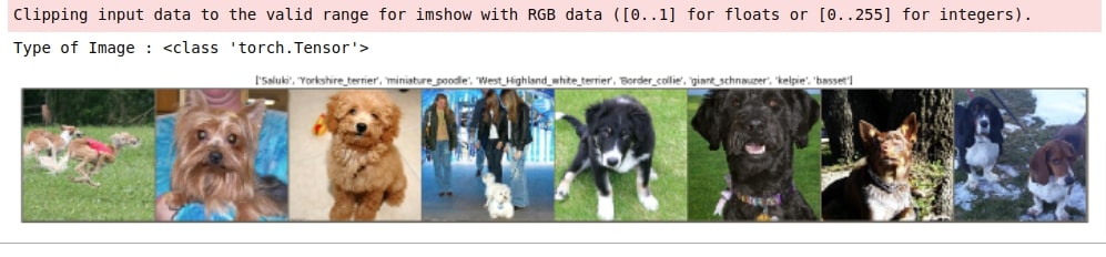
Visualizing Train Images
Below we are visualizing the first batch which consists of 8 images from the training dataset to get an idea of images.
images,labels = next(iter(loaders['train']))
inp = torchvision.utils.make_grid(images)
print('Type of Image : '+ str(type(inp)))
inp = inp.numpy().transpose(1,2,0)
mean = np.array([0.485, 0.456, 0.406])
std = np.array([0.229, 0.224, 0.225])
image = std * inp + mean
iamge = image.clip(0,1)
plt.figure(figsize=(25,5))
plt.imshow(image)
plt.title(str([idx_to_dog_breed[label].split('-')[1] for label in labels.numpy()]))
plt.xticks([])
plt.yticks([])
None
Loading Model with Pretrained Weights
Pytorch provides different module by name of torchvision for providing some pre-trained image classification models and few image manipulation functionalities.
We'll be using VGG neural network which was 1st runner up at ILSVRC (ImageNet Large Scale Visual Recognition Competition) 2014. It's designed by the Visual Geometry Group of Oxford University.
VGG neural network has quite a simple structure compared to other competition winner neural networks and also quite good performance. It first used 3x3 convolution for training and many other models are based on it hence worth exploring.
vgg = models.vgg16(pretrained=True)
for param in list(vgg.parameters())[:-1]:
    param.requires_grad = False
vgg.classifier[6] = nn.Linear(4096, len(dog_breeds))
vgg = vgg.to(device)
vgg
Initializing Loss Function and Optimization Function
Below we have defined CrossEntropyLoss function which we'll be optimizing and Stochastic Gradient Descent Optimizer initialized with a parameter of VGG neural net & learning rate of 0.001.
loss_function = nn.CrossEntropyLoss()
optimizer = optim.SGD(params=vgg.parameters(), lr = 0.001)
Model Training
Below we have defined function which we'll be using for training providing it epochs for it should run. One epoch refers to one pass through whole training data to train the neural network and one pass through validation data to check accuracy.
def train(epochs):
    for epoch in range(epochs):
        for phase in ['train', 'val']:
            if phase == 'train':
                vgg.train() ## We set model to train phase as it activates layers like Dropout and BatchNormalization.
            else:
                vgg.eval() ## We set model to train phase as it de-activates layers like Dropout and BatchNormalization.

            total_loss = 0.0
            correct_preds = 0

            for i, (images, labels) in enumerate(loaders[phase]):
                images, labels = images.to(device), labels.to(device) ## Translate normal tensor to cuda tensors it GPU is available.
                optimizer.zero_grad() ## At start of each batch we set gradients of loss with respect to parameters to zero.
                with torch.set_grad_enabled(phase == 'train'): ## This enables gradients calculation based on phase.
                    results = vgg.forward(images) ## We do forward pass thorugh batch images.
                    _, predictions = torch.max(results,1) ## We get indexes of max probabilities for each image of batch.
                    loss = loss_function(predictions, labels) ## We calculation loss based on predicted probabilities and actual ones.

                    if phase == 'train':
                        loss.backward() # Backpropogation execution which calculates gradients for each weight parameter.
                        optimizer.step() ## This step updates weights based on gradients calculated above and learning rate set above.
                #print(i)
                total_loss += loss.item()
                correct_preds += torch.sum(predictions == labels) ## We find out correct predictions.

            print('Epoch : %d'%(epoch+1))
            print('Stage : %s'%phase)
            print('Loss : %f'%total_loss)
            #print(correct_preds.item())
            print('Accuracy : %f'% (int(correct_preds.item()) / len(dsets[phase])))
            print('-'*100)
Below we are a training model for 3 epochs and check accuracy for training and validation data.
%time train(3)
We execute training for 2 more epochs to check whether it still improves accuracy.
%time train(2)
We train for 2 more epochs with the same learning rate to check whether it's still improving accuracy.
%time train(2)
We noticed above that accuracy is not improving hence we are reducing the learning rate and then will train for 2 more epochs to check whether it improves accuracy.
optimizer.lr = 0.0001
%time train(2)
Model Testing
We now have an accuracy of almost 85+%. We'll now test our model on test data which we have kept aside for the final round of testing.
def test():
    with torch.no_grad(): ## We are setting it to no grads as we don't need gradients during testing.
        correct = 0
        #loss = 0
        for images,labels in loaders['test']:
            images,labels = images.to(device), labels.to(device)

            predictions = vgg(images)
            _, preds = torch.max(predictions, 1)
            correct += torch.sum(preds == labels)
        print('Test Set Accuracy : %f'%(correct.item() / len(dsets['test'])))

%time test()
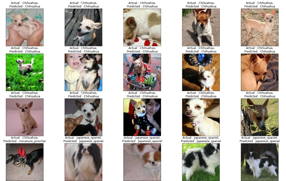
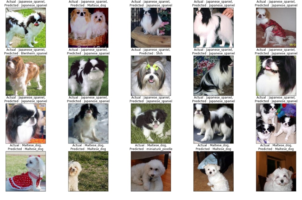
Visualizing Predictions on Test Data
Below we have written function which visualizes the first 40 images of test images.
def visualizing_predictions_on_test_data():
    plt.figure(figsize=(22,28))
    with torch.no_grad():
        for i, (image,label) in enumerate(loaders['test']):
            if i == 40:
                break
            plt.subplot(8,5,i+1)
            image,label = image.to(device), label.to(device)

            prediction = vgg(image)
            _, pred = torch.max(prediction,1)
            img = image.to('cpu').numpy()[0].transpose(1,2,0)
            mean = np.array([0.485, 0.456, 0.406])
            std = np.array([0.229, 0.224, 0.225])
            img = std * img + mean
            plt.imshow(img.clip(0.0,1.0))
            plt.title('Actual : %s,\nPredicted : %s'%(idx_to_dog_breed[int(label.item())].split('-')[1], idx_to_dog_breed[int(pred.item())].split('-')[1]))
            plt.xticks([])
            plt.yticks([])

visualizing_predictions_on_test_data()
Finetuning Convnet:
We'll now try finetuning the VGG model. Here we'll replace the last Linear Layer with our requirements so that it outputs 120 probabilities for each image instead of 1000 for Imagenet. We then proceed to train with this model.
Note: Here requires_grad is True for all parameters hence all layers will be trained. We have set only the last Linear layer as True in fixed feature extractor type of transfer learning.
vgg = models.vgg16(pretrained=True)
vgg.classifier[6] = nn.Linear(4096, len(dog_breeds))
vgg = vgg.to(device)
vgg
Please make a note here that we have set a learning rate as low as 0.0001 because we don't want to mess up nicely trained Convolution Layer's weights much. We just want to fine-tune them a little bit.
loss_function = nn.CrossEntropyLoss()
optimizer = optim.SGD(params=vgg.parameters(), lr = 0.0001)
%time train(3)
 Sunny Solanki
Sunny Solanki
Intro: Software Developer | Youtuber | Bonsai Enthusiast
About: Sunny Solanki holds a bachelor's degree in Information Technology (2006-2010) from L.D. College of Engineering. Post completion of his graduation, he has 8.5+ years of experience (2011-2019) in the IT Industry (TCS). His IT experience involves working on Python & Java Projects with US/Canada banking clients. Since 2020, he’s primarily concentrating on growing CoderzColumn.
His main areas of interest are AI, Machine Learning, Data Visualization, and Concurrent Programming. He has good hands-on with Python and its ecosystem libraries.
Apart from his tech life, he prefers reading biographies and autobiographies. And yes, he spends his leisure time taking care of his plants and a few pre-Bonsai trees.
Contact: sunny.2309@yahoo.in


![YouTube Subscribe]() Comfortable Learning through Video Tutorials?
Comfortable Learning through Video Tutorials?
If you are more comfortable learning through video tutorials then we would recommend that you subscribe to our YouTube channel.
![Need Help]() Stuck Somewhere? Need Help with Coding? Have Doubts About the Topic/Code?
Stuck Somewhere? Need Help with Coding? Have Doubts About the Topic/Code?
 Stuck Somewhere? Need Help with Coding? Have Doubts About the Topic/Code?
When going through coding examples, it's quite common to have doubts and errors.
If you have doubts about some code examples or are stuck somewhere when trying our code, send us an email at coderzcolumn07@gmail.com. We'll help you or point you in the direction where you can find a solution to your problem.
You can even send us a mail if you are trying something new and need guidance regarding coding. We'll try to respond as soon as possible.
![Share Views]() Want to Share Your Views? Have Any Suggestions?
Want to Share Your Views? Have Any Suggestions?
 Want to Share Your Views? Have Any Suggestions?
If you want to
- provide some suggestions on topic
- share your views
- include some details in tutorial
- suggest some new topics on which we should create tutorials/blogs
 transfer-learning, pytorch