Explain Text Classification Models Using SHAP Values (Keras + Vectorized Data)
SHAP (SHapley Additive exPlanations) is a Python library that generates SHAP values using the game-theoretic approach that can be used to explain predictions of our deep learning models. It provides different kinds of explainers that use different algorithms to generate shap values for features of our data to explain the prediction of our model. This can be very helpful in getting insights into predictions made by our model. We can dig deep to understand whether the predictions made by our model make sense and whether it's generating predictions by using correct parts of data which we expect should be used to make a decision or as a tie-breaker.
We have already covered a detailed tutorial on SHAP where we have explained how it can be used with tabular data and scikit-learn models. Please feel free to check the below link if you want to go through it as we have included a detailed intro to SHAP library there.
As a part of this tutorial, we'll use SHAP to explain predictions made by our text classification model. We have used 20 newsgroups dataset available from scikit-learn for our task. We have vectorized text data to a list of floats using the Tf-Idf approach. We have used the keras model to classify text documents into various categories. Once the model is trained and gives good accuracy, we have explained the predictions using SHAP explainers (Partition Explainer and Permutation Explainer).
We have one more tutorial explaining how to use shap values for the text classification tasks. In that tutorial, we have used the keras text vectorization layer to vectorize text data instead of the scikit-learn vectorizer that we have used in this tutorial. Please feel free to check if you are using the keras text vectorization layer in your task.
Below, we have listed important sections of tutorial to give an overview of the material covered.
Important Sections Of Tutorial
- Load Data
- Vectorize Data
- Define Model
- Compile And Train Model
- Evaluate Model Performance
- Explain Model Predictions Using SHAP Partition Explainer
- Visualize SHAP Values Correct Predictions
- Text Plot
- Bar Chart
- Waterfall Chart
- Force Plot
- Visualize SHAP Values Incorrect Predictions
- Visualize SHAP Values Correct Predictions
- Explain Model Predictions Using SHAP Permutation Explainer
Below, we have imported the main libraries of the tutorial and printed the versions that we have used.
import tensorflow
from tensorflow import keras

print("Keras Version : {}".format(keras.__version__))
import shap

print("SHAP Version : {}".format(shap.__version__))
1. Load Data 
In this section, we have loaded our 20-newsgroups text dataset available from scikit-learn. It has nearly 18k text documents for 20 different categories. For our tutorial, we have limited text documents of only 5 categories listed below in code. We have loaded dataset using fetch_20newsgroups() function of datasets sub-module of scikit-learn. It let us load train and test sets separately.
import numpy as np
from sklearn import datasets

all_categories = ['alt.atheism','comp.graphics','comp.os.ms-windows.misc','comp.sys.ibm.pc.hardware',
                  'comp.sys.mac.hardware','comp.windows.x', 'misc.forsale','rec.autos','rec.motorcycles',
                  'rec.sport.baseball','rec.sport.hockey','sci.crypt','sci.electronics','sci.med',
                  'sci.space','soc.religion.christian','talk.politics.guns','talk.politics.mideast',
                  'talk.politics.misc','talk.religion.misc']

selected_categories = ['alt.atheism','comp.graphics','rec.motorcycles','sci.space','talk.politics.misc']

X_train_text, Y_train = datasets.fetch_20newsgroups(subset="train", categories=selected_categories, return_X_y=True)
X_test_text , Y_test  = datasets.fetch_20newsgroups(subset="test", categories=selected_categories, return_X_y=True)

X_train_text = np.array(X_train_text)
X_test_text = np.array(X_test_text)

classes = np.unique(Y_train)
mapping = dict(zip(classes, selected_categories))

len(X_train_text), len(X_test_text), classes, mapping
2. Vectorize Text Data 
In this section, we have vectorized our text data i.e., convert text documents to a list of floats. There are various text vectorization approaches but as a part of this tutorial we have used Tf-IDF (Term Frequency - Inverse Document Frequency) approach which generates float per word in a text document in a way that words appear commonly across all documents gets low values and those appearing rarely across documents gets more value. This approach can help us get better accuracy with our data. We'll be training our network later on this vectorized data.
We have vectorized data using TidfVectorizer() estimator available from scikit-learn.
If you want to know in-depth how text vectorization works then please feel free to check the below link. It explains concepts with simple examples.
Please feel free to check the below link if you want to learn about text classification using keras.
import sklearn
import numpy as np
from sklearn.feature_extraction.text import CountVectorizer, TfidfVectorizer

vectorizer = TfidfVectorizer(max_features=50000)

vectorizer.fit(np.concatenate((X_train_text, X_test_text)))
X_train = vectorizer.transform(X_train_text)
X_test = vectorizer.transform(X_test_text)

X_train, X_test = X_train.toarray(), X_test.toarray()

X_train.shape, X_test.shape
import gc

gc.collect()
3. Define Model 
In this section, we have defined the neural network that we'll use for the text classification task. It has 3 dense layers with units 128, 64, and 5 (number of target classes). The first two dense layers have relu (rectified linear unit) activation and the last dense layer have softmax activation. We have created a small function that creates and returns a network.
from tensorflow.keras.models import Sequential
from tensorflow.keras import layers

def create_model():
    return Sequential([
                        layers.Input(shape=X_train.shape[1:]),
                        layers.Dense(128, activation="relu"),
                        layers.Dense(64, activation="relu"),
                        layers.Dense(len(classes), activation="softmax"),
                    ])

model = create_model()

model.summary()
4. Compile And Train Model 
In this section, we have first compiled the network to use Adam optimizer, cross entropy loss, and accuracy metric. Then, we have trained the network for 5 epochs using train data. We can notice from the results that the model has reasonably good accuracy after 5 epochs.
model.compile("adam", "sparse_categorical_crossentropy", metrics=["accuracy"])
history = model.fit(X_train, Y_train, batch_size=256, epochs=5, validation_data=(X_test, Y_test))
gc.collect()
5. Evaluate Model Performance 
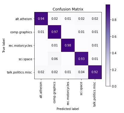
In this section, we have evaluated the performance of the network by calculating accuracy, classification report (precision, recall, and f1-score per target category) and confusion matrix metrics on test predictions. We can notice from the classification report that 'talk.politics.misc' category has a little less accuracy compared to other categories. The few samples of 'talk.politics.misc' are confused with 'sci.space' and few samples of 'sci.space' are confused with 'comp.graphics' per confusion matrix.
from sklearn.metrics import accuracy_score, classification_report

train_preds = model.predict(X_train)
test_preds = model.predict(X_test)

print("Train Accuracy : {:.3f}".format(accuracy_score(Y_train, np.argmax(train_preds, axis=1))))
print("Test  Accuracy : {:.3f}".format(accuracy_score(Y_test, np.argmax(test_preds, axis=1))))
print("\nClassification Report : ")
print(classification_report(Y_test, np.argmax(test_preds, axis=1), target_names=selected_categories))
from sklearn.metrics import confusion_matrix
import scikitplot as skplt
import matplotlib.pyplot as plt

skplt.metrics.plot_confusion_matrix([selected_categories[i] for i in Y_test], [selected_categories[i] for i in np.argmax(test_preds, axis=1)],
                                    normalize=True,
                                    title="Confusion Matrix",
                                    cmap="Purples",
                                    hide_zeros=True,
                                    figsize=(5,5)
                                    );
plt.xticks(rotation=90);
6. SHAP Partition Explainer 
In this section, we have explained the predictions made by our model using the SHAP Partition explainer. It recursively tries a hierarchy of features to determine shap values. We have generated shap values for correct predictions as well as incorrect predictions to better understand which words contributed to each type of prediction.
In order to use SHAP, we need to initialize it first by calling initjs() function. Then, we have created a Partition explainer using Explainer() constructor. We'll be using this explainer to generate shap values for our predictions. We need to give function or model (takes text data as input and makes predictions) and masker as input to the constructor.
We have first designed a function that takes text data samples as input and returns predictions. It first vectorizes data using the vectorizer we created earlier and then makes predictions.
The masker is generally used internally by shap functions to hide parts of the text for which we don't have shape values like punctuations, spaces between words, etc. We have created a masker using Text() constructor by providing regular expression pattern 'r"\W+"'. When we provide a regular expression like this, the constructor internally creates a tokenizer using it. We can also create our tokenizer function and provide it to this masker. The tokenizer should return a dictionary with two keys.
- 'input_ids' - The value of this key should be a list of tokens that are not words. It is tokens that are between words like punctuations, spaces, etc. The tokens separate two words.
- 'offset_mapping' - The values of this key should be a list of tuples of length two. These tuples are start and end indexes of tokens available in 'input_ids' values.
When we create a masker using the regular expression 'r"\W+"', it'll internally create a dictionary with the above keys.
Please make a NOTE that even if we don't provide a pattern when creating a masker object, it'll still use the same 'r"\W+"' pattern.
shap.initjs()

def make_predictions(X_batch_text):
    X_batch = vectorizer.transform(X_batch_text).toarray()
    preds = model.predict(X_batch)
    return preds

masker = shap.maskers.Text(tokenizer=r"\W+")
explainer = shap.Explainer(make_predictions, masker=masker, output_names=selected_categories)

explainer
Visualize SHAP Values Correct Predictions 
In this section, we have generated shap values for correct predictions and created visualizations using those shap values.
Below, we have first selected two samples from test data and printed their contents. Then, we have made predictions on them using our model. We have printed the actual label, target label, and probabilities for them. The first category is 'sci.space' and second is 'alt.atheism'. Both are predicted correctly by our model with probabilities 0.91 and 0.79 respectively.
We have then calculated SHAP values by calling the explainer object with data samples. We have also printed the shape of base values and shap values in the next cell after the below cell.
import re

X_batch_text = X_test_text[1:3]
X_batch = X_test[1:3]

print("Samples : ")
for text in X_batch_text:
    print(re.split(r"\W+", text))
    print()

preds_proba = model.predict(X_batch)
preds = preds_proba.argmax(axis=1)

print("Actual    Target Values : {}".format([selected_categories[target] for target in Y_test[1:3]]))
print("Predicted Target Values : {}".format([selected_categories[target] for target in preds]))
print("Predicted Probabilities : {}".format(preds_proba.max(axis=1)))

shap_values = explainer(X_batch_text)
print("SHAP Values Shape : {}".format(shap_values.shape))
print("SHAP Base Values  : {}".format(shap_values.base_values))
print("SHAP Data : ")
print(shap_values.data[0])
print(shap_values.data[1])
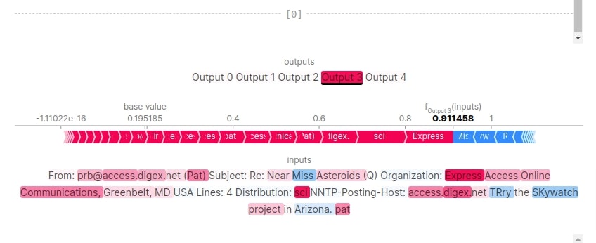
Text Plot
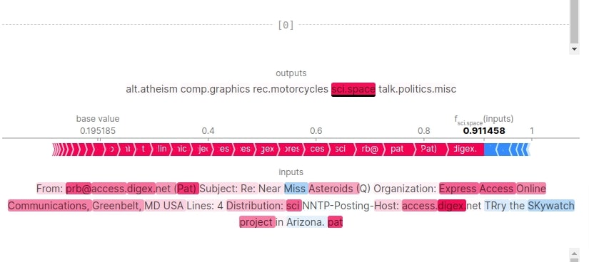
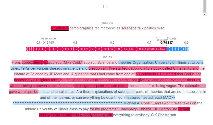
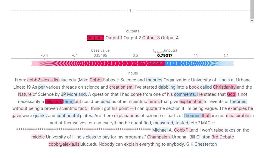
In this section, we have created a text plot using shap values. The text plot shows actual text content whose words are color-coded based on their shap values. The words that contribute positively are color-coded as shaded of red and words that contribute negatively are color-coded shades of blue.
We can notice from the output of the first sample that words like 'asteroids', 'communications', 'greenbelt', 'sci', etc have contributed to predicting category 'sci.space'. For second samples, words like 'religious', 'creationism', 'Christianity', 'god', etc has contributed positively to predicting category 'alt.atheism'. There are also words that contributed negatively to predictions.
The visualization is interactive and we can click on other categories as well to see which words in our text have contributed to those categories as well.
shap.text_plot(shap_values)
Bar Chart
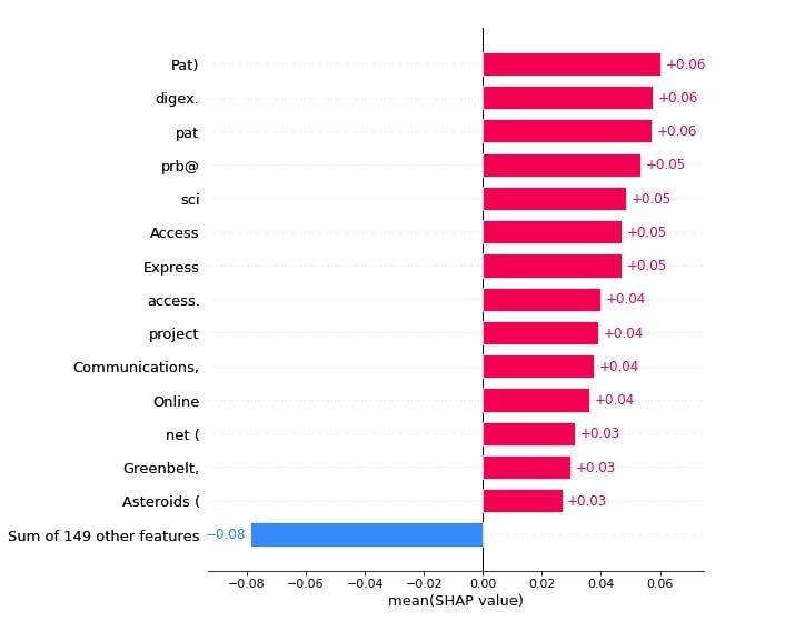
In this section, we have created various bar charts showing the importance of words to predictions. We can create bar charts using bar() function.
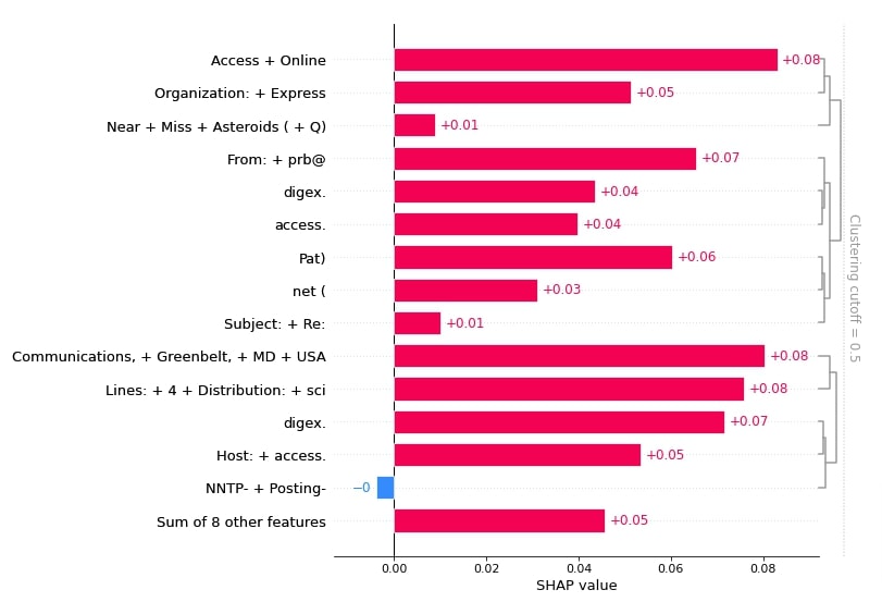
Below, we have created a bar chart showing the shap values of words that contributed to predicting category 'sci.space'. Please pay close attention to how we have provided shap values to different functions.
shap.plots.bar(shap_values[:,:, selected_categories[preds[0]]].mean(axis=0), max_display=15,
               order=shap.Explanation.argsort.flip)
Below, we have created another bar chart showing shap values of words from 1st samples that contributed to predicting category 'sci.space'.
shap.plots.bar(shap_values[0,:, selected_categories[preds[0]]], max_display=15,
               order=shap.Explanation.argsort.flip)
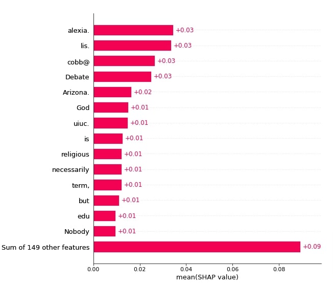
Below, we have created a bar chart showing the shap values of words that contributed to predicting category 'alt.atheism'.
shap.plots.bar(shap_values[:,:, selected_categories[preds[1]]].mean(axis=0), max_display=15,
               order=shap.Explanation.argsort.flip)
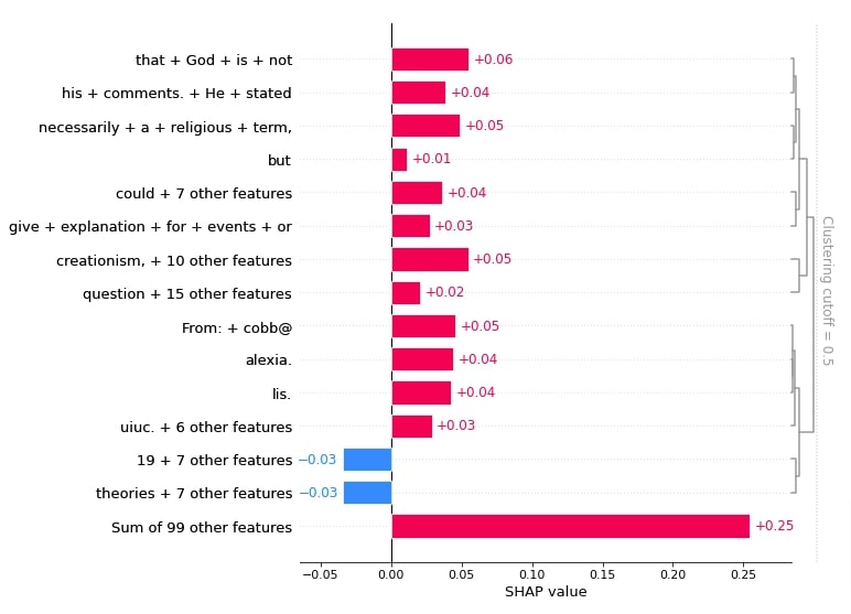
Below, we have created a bar chart showing shap values of words from the 2nd sample that contributed to predicting category 'alt.atheism'.
shap.plots.bar(shap_values[1,:, selected_categories[preds[1]]], max_display=15,
               order=shap.Explanation.argsort.flip)
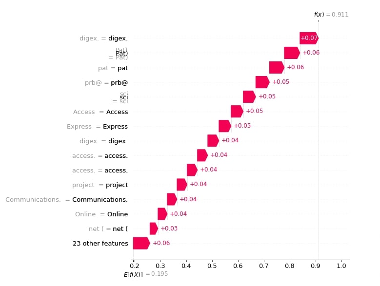
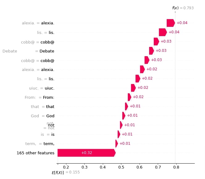
Waterfall Plot
In this section, we have created a waterfall chart for shap values. The waterfall chart shows how adding shap values to base value generates prediction probability. We can create a waterfall chart using waterfall_plot() function available from SHAP.
Below, we have created waterfall plots for the first and second samples respectively.
shap.waterfall_plot(shap_values[0][:, selected_categories[preds[0]]], max_display=15)
shap.waterfall_plot(shap_values[1][:, selected_categories[preds[1]]], max_display=15)
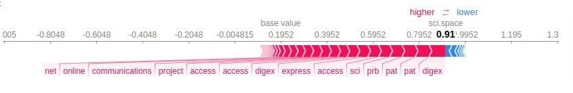
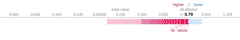
Force Plot
In this section, we have created a force plot that shows how adding shap values to base values generates predictions just like a waterfall chart but the layout used for the plot is additive force layout.
Below, we have created a force plot for both of our predictions using their respective shap values. Please pay close attention to how we have provided base values and shap values to force_plot() function.
print(selected_categories)
import re

tokens = re.split("\W+", X_batch_text[0].lower())

shap.force_plot(shap_values.base_values[0][preds[0]], shap_values[0][:, preds[0]].values,
                feature_names = tokens[:-1], out_names=selected_categories[preds[0]])
import re

tokens = re.split("\W+", X_batch_text[1].lower())

shap.force_plot(shap_values.base_values[1][preds[1]], shap_values[1][:, preds[1]].values,
                feature_names = tokens[:-1], out_names=selected_categories[preds[1]])
Visualize SHAP Values Incorrect Predictions 
In this section, we are analyzing shap values for wrong predictions. This will help us understand which words contributed to wrong predictions for our samples.
To find out wrong predictions, we have first made predictions for all test samples and compared them with actual target values of test samples to find our indexes of samples that were predicted wrong. Then, we have taken 2 samples that were predicted wrong by our model.
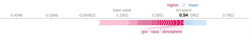
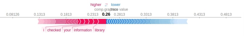
For first sample, the actual category is 'talk.politics.misc' but our model predicted 'sci.space' with probability of 0.54. For second samples, the actual category is 'alt.atheism' but our model predicted 'comp.graphics' with probability of 0.25.
We have generated shap values for both samples by using the explainer object we created earlier. We have also printed the shape of base values and shap values in the next cell.
import re

Y_test_preds = model.predict(X_test)
Y_test_preds = Y_test_preds.argmax(axis=1)

wrong_preds = np.argwhere(Y_test!=Y_test_preds)
X_batch_text = X_test_text[wrong_preds.flatten()[:2]]
X_batch = X_test[wrong_preds.flatten()[:2]]

print("Samples : ")
for text in X_batch_text:
    print(re.split(r"\W+", text))
    print()

preds_proba = model.predict(X_batch)
preds = preds_proba.argmax(axis=1)

print("Actual    Target Values : {}".format([selected_categories[target] for target in Y_test[wrong_preds.flatten()[:2]]]))
print("Predicted Target Values : {}".format([selected_categories[target] for target in preds]))
print("Predicted Probabilities : {}".format(preds_proba.max(axis=1)))

shap_values = explainer(X_batch_text)

shap_values.shape
print("SHAP Values Shape : {}".format(shap_values.shape))
print("SHAP Base Values  : {}".format(shap_values.base_values))
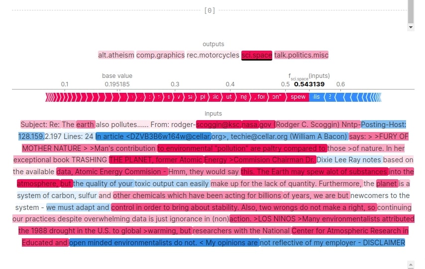
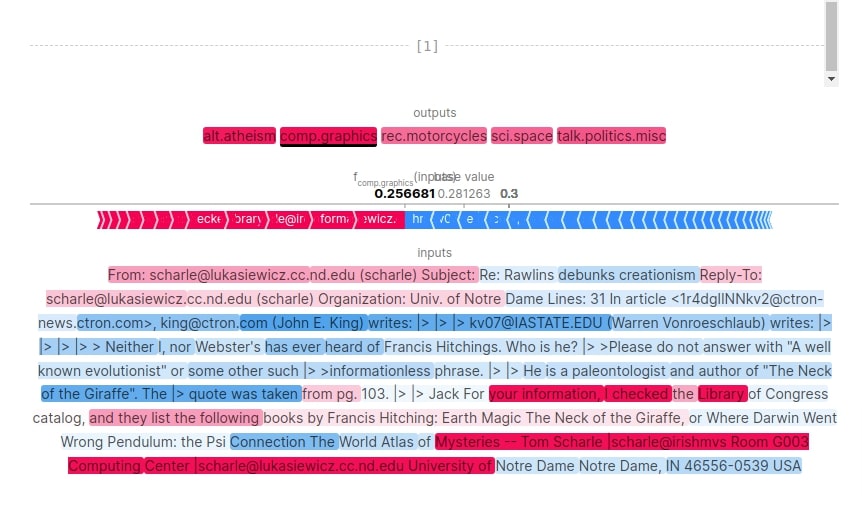
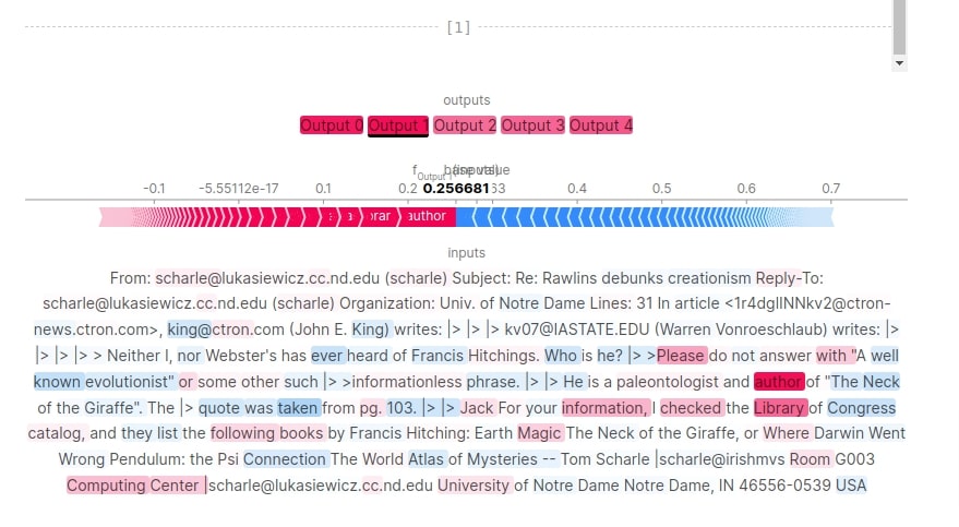
Text Plot
Below, we have generated a text plot using the shap values of our samples. We can notice that the first sample had a word like 'planet', 'earth', 'atmosphere', etc which could have contributed to predicting category 'sci.space' instead of 'talk.politics.misc'. For second samples, our model is very much confused between 'comp.graphics' and 'alt.atheism' as probabilities of them is 0.25 and 0.24 respectively which is very close.
shap.text_plot(shap_values)
Bar Chart
In this section, we have created various bar charts showing words that contributed to wrong predictions.
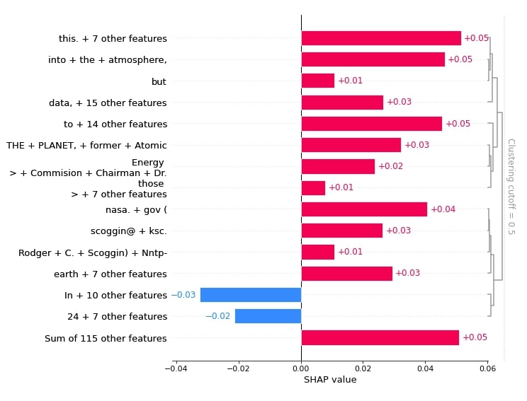
Below, we have generated a bar chart showing shap values of words from 1st sample that contributed to predicting category 'sci.space'.
shap.plots.bar(shap_values[0,:, selected_categories[preds[0]]], max_display=15,
               order=shap.Explanation.argsort.flip)
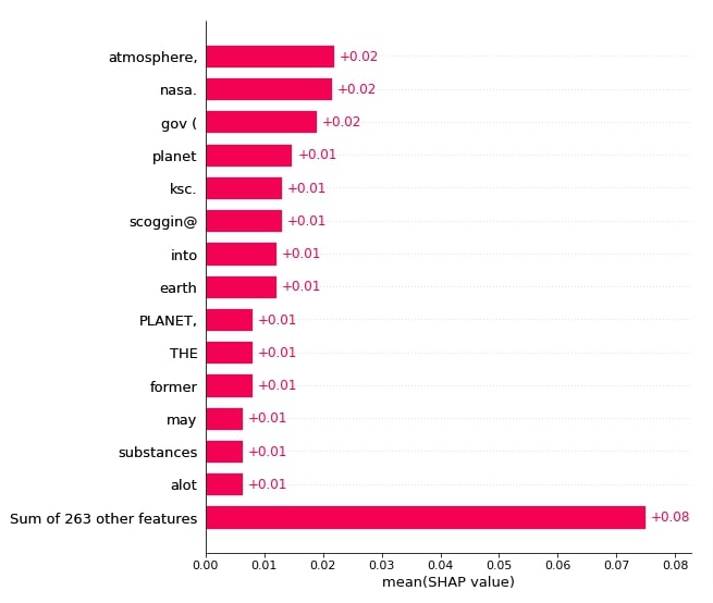
Below, we have generated a bar chart showing shap values of words that contributed to predicting category 'sci.space'.
shap.plots.bar(shap_values[:,:, selected_categories[preds[0]]].mean(axis=0), max_display=15,
               order=shap.Explanation.argsort.flip)
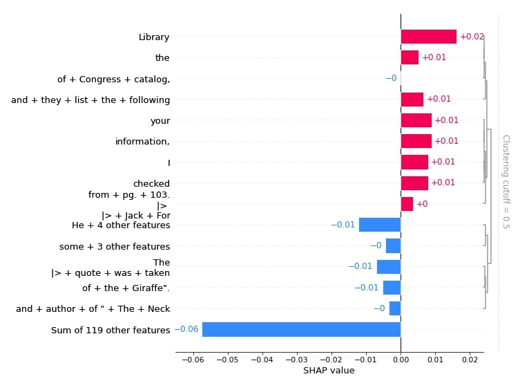
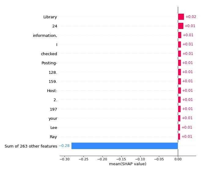
Below, we have created a bar chart showing shap values of words from 2nd samples that contributed predicting category 'comp.graphics'.
shap.plots.bar(shap_values[1,:, selected_categories[preds[1]]], max_display=15,
               order=shap.Explanation.argsort.flip)
Below, we have created a bar chart showing the shap values of words that contributed to predicting category 'comp.graphics'.
shap.plots.bar(shap_values[:,:, selected_categories[preds[1]]].mean(axis=0), max_display=15,
               order=shap.Explanation.argsort.flip)
Force Plot
In this section, we have created force plots for both wrong predictions one after another.
print(selected_categories)
import re

tokens = re.split("\W+", X_batch_text[0].lower())

shap.force_plot(shap_values.base_values[0][preds[0]], shap_values[0][:, preds[0]].values,
                feature_names = tokens[:-1], out_names=selected_categories[preds[0]])
import re

tokens = re.split("\W+", X_batch_text[1].lower())

shap.force_plot(shap_values.base_values[1][preds[1]], shap_values[1][:, preds[1]].values,
                feature_names = tokens[:-1], out_names=selected_categories[preds[1]])
7. SHAP Permutation Explainer 
In this section, we have used Permutation explainer to explain predictions made by our model. Just like previous sections, we have tried to explain both correct and incorrect predictions. Permutation explainer iterates through all permutation of features in forward and reverse direction to generate shap values. This explainer can sometimes take time if tried with many samples.
Below, we have created a permutation explainer using PermutationExplainer() constructor available from the SHAP library. We have provided the same parameters to it that we had provided to the partition explainer. We'll be using this explainer instance to generate shap values which will be visualized to better understand predictions.
def make_predictions(X_batch_text):
    X_batch = vectorizer.transform(X_batch_text).toarray()
    preds = model.predict(X_batch)
    return preds

masker = shap.maskers.Text(tokenizer=r"\W+")
explainer = shap.PermutationExplainer(make_predictions, masker=masker, output_names=selected_categories)

explainer
Visualize SHAP Values For Correct Predictions 
In this section, we are explaining the correct predictions made by our model. We have taken two samples from our data and made predictions on them using our trained model. The first sample is correctly predicted as 'sci.space' category with a probability of 0.91 and the second sample is correctly predicted as 'alt.atheism' category with the probability of 0.79. We have also displayed tokenized content of the text documents.
Then, we have generated shap values for both samples using our permutation explainer.
In the next cell below, we have printed base values and shape of shap values.
import re

X_batch_text = X_test_text[1:3]
X_batch = X_test[1:3]

print("Samples : ")
for text in X_batch_text:
    print(re.split(r"\W+", text))
    print()

preds_proba = model.predict(X_batch)
preds = preds_proba.argmax(axis=1)

print("Actual    Target Values : {}".format([selected_categories[target] for target in Y_test[1:3]]))
print("Predicted Target Values : {}".format([selected_categories[target] for target in preds]))
print("Predicted Probabilities : {}".format(preds_proba.max(axis=1)))

shap_values = explainer(X_batch_text)
print("SHAP Values Shape : {}".format(shap_values.shape))
print("SHAP Base Values  : {}".format(shap_values.base_values))
Text Plot
Here, we have generated a text plot to see which words contributed to predicting categories correctly.
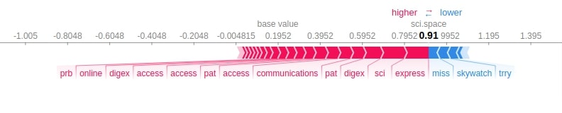
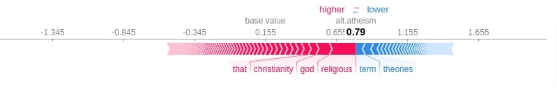
For first sample, words like 'sci', 'communications', 'express', etc has contributed to predicting category 'sci.space'. For second sample, words like 'god', 'religious', 'Christianity', 'creationism', etc has contributed to predicting category 'alt.atheism'.
print(selected_categories)
shap.text_plot(shap_values)
Force Plot
In this section, we have created force plots for the first and second samples using their respective shap values.
print(selected_categories)
import re

tokens = re.split("\W+", X_batch_text[0].lower())

shap.force_plot(shap_values.base_values[0][preds[0]], shap_values[0][:, preds[0]].values,
                feature_names = tokens[:-1], out_names=selected_categories[preds[0]])
import re

tokens = re.split("\W+", X_batch_text[1].lower())

shap.force_plot(shap_values.base_values[1][preds[1]], shap_values[1][:, preds[1]].values,
                feature_names = tokens[:-1], out_names=selected_categories[preds[1]])
Visualize SHAP Values For Incorrect Predictions 
In this section, we'll use our explainer to understand the wrong predictions made by our model.
First, we have found out indexes of wrong test predictions like earlier. Then, we have selected two samples that are predicted wrong and made predictions on them. For first sample, actual category is 'talk.politics.misc' but model predicted 'sci.space' with probability 0.54 and for second sample, actual category is 'alt.atheism' but our model predicted 'comp.graphics' with probability 0.25.
We have generated shap values for both samples using our explainer object as usual.
import re

Y_test_preds = model.predict(X_test)
Y_test_preds = Y_test_preds.argmax(axis=1)

wrong_preds = np.argwhere(Y_test!=Y_test_preds)
X_batch_text = X_test_text[wrong_preds.flatten()[:2]]
X_batch = X_test[wrong_preds.flatten()[:2]]

print("Samples : ")
for text in X_batch_text:
    print(re.split(r"\W+", text))
    print()

preds_proba = model.predict(X_batch)
preds = preds_proba.argmax(axis=1)

print("Actual    Target Values : {}".format([selected_categories[target] for target in Y_test[wrong_preds.flatten()[:2]]]))
print("Predicted Target Values : {}".format([selected_categories[target] for target in preds]))
print("Predicted Probabilities : {}".format(preds_proba.max(axis=1)))

shap_values = explainer(X_batch_text)

shap_values.shape
print("SHAP Values Shape : {}".format(shap_values.shape))
print("SHAP Base Values  : {}".format(shap_values.base_values))
Text Plot
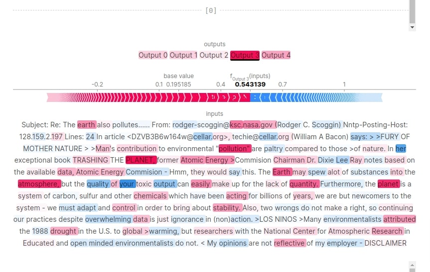
In this section, we have generated text plot visualization using shap values to see which words contributed to wrong predictions.
For the first sample, we can notice from the visualization that words like 'planet', 'atmosphere', 'earth', etc have contributed to predicting category 'sci.space'. Though the model was not much sure (0.54 probability) about it due to the presence of some words related to politics like 'environmental', 'energy', 'environmentalists', 'opinions', etc.
For second sample, the model is very much confused between 'comp.graphics' and 'alt.atheism'. The presence of words like 'author', 'books', 'computing center', 'information', etc has led it to predict 'comp.graphics'. Though the probability of 'comp.graphics' is 0.25 and probability of 'alt.atheism' is 0.24 which is very minor difference.
shap.text_plot(shap_values)
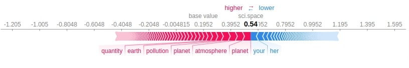
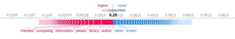
Force Plot
In this section, we have created force plots explaining the first and second samples.
print(selected_categories)
import re

tokens = re.split("\W+", X_batch_text[0].lower())

shap.force_plot(shap_values.base_values[0][preds[0]], shap_values[0][:, preds[0]].values, feature_names = tokens[:-1], out_names=selected_categories[preds[0]])
import re

tokens = re.split("\W+", X_batch_text[1].lower())

shap.force_plot(shap_values.base_values[1][preds[1]], shap_values[1][:, preds[1]].values, feature_names = tokens[:-1], out_names=selected_categories[preds[1]])
This ends our small tutorial explaining how we can explain the predictions made by Flax (JAX) text classification network using SHAP values. Please feel free to let us know your views in the comments section.
References
 Sunny Solanki
Sunny Solanki
Intro: Software Developer | Youtuber | Bonsai Enthusiast
About: Sunny Solanki holds a bachelor's degree in Information Technology (2006-2010) from L.D. College of Engineering. Post completion of his graduation, he has 8.5+ years of experience (2011-2019) in the IT Industry (TCS). His IT experience involves working on Python & Java Projects with US/Canada banking clients. Since 2020, he’s primarily concentrating on growing CoderzColumn.
His main areas of interest are AI, Machine Learning, Data Visualization, and Concurrent Programming. He has good hands-on with Python and its ecosystem libraries.
Apart from his tech life, he prefers reading biographies and autobiographies. And yes, he spends his leisure time taking care of his plants and a few pre-Bonsai trees.
Contact: sunny.2309@yahoo.in


![YouTube Subscribe]() Comfortable Learning through Video Tutorials?
Comfortable Learning through Video Tutorials?
If you are more comfortable learning through video tutorials then we would recommend that you subscribe to our YouTube channel.
![Need Help]() Stuck Somewhere? Need Help with Coding? Have Doubts About the Topic/Code?
Stuck Somewhere? Need Help with Coding? Have Doubts About the Topic/Code?
 Stuck Somewhere? Need Help with Coding? Have Doubts About the Topic/Code?
When going through coding examples, it's quite common to have doubts and errors.
If you have doubts about some code examples or are stuck somewhere when trying our code, send us an email at coderzcolumn07@gmail.com. We'll help you or point you in the direction where you can find a solution to your problem.
You can even send us a mail if you are trying something new and need guidance regarding coding. We'll try to respond as soon as possible.
![Share Views]() Want to Share Your Views? Have Any Suggestions?
Want to Share Your Views? Have Any Suggestions?
 Want to Share Your Views? Have Any Suggestions?
If you want to
- provide some suggestions on topic
- share your views
- include some details in tutorial
- suggest some new topics on which we should create tutorials/blogs
 shap-values, text-classification, keras