MXNet: CNNs With Conv1D for Text Classification Tasks
Text data is a type of data that has a sequence in it. We need to follow the grammar of the language in order to create sentences and it requires a sequence of words to appear in a particular sequence. Due to this, when we are trying to solve any NLP task using neural networks, it is preferable that we design a network that can capture the sequence of text. This kind of network that can capture sequences gives the best results. The commonly used deep neural networks which consist of only dense/linear layers are not good at this. Recurrent neural networks are the ones that are specifically designed for this purpose and do a very good job at capturing a sequence of data. But some research has shown that we can use convolutional neural networks with 1D convolution layers as well for NLP tasks and it can give good results as well. Hence, we'll be concentrating on them in this tutorial.
As a part of this tutorial, we have explained how we can create CNNs consisting of 1D Convolution (Conv1D) layers using MXNet for solving text classification tasks. MXNet is a python deep learning library for creating neural networks designed by Apache. We'll be using word embeddings approach to encoding text data to real-valued data as required by networks. We have also evaluated the performance of CNNs by calculating various ML metrics and also explained predictions made by them using LIME algorithms to better understand them.
Below, we have listed essential sections of tutorial to give an overview of the material covered.
Important Sections Of Tutorial
- Prepare Data
- 1.1 Load Dataset
- 1.2 Define Tokenizer
- 1.3 Build Vocabulary
- 1.4 Define Vectorization Function
- 1.5 Create Data Loaders
- Approach 1: Single Conv1D Layer Network (Max Tokens=50, Embedding Length=128, Conv Output Channels=32)
- Define Convolutional Neural Network
- Train Network
- Evaluate Network Performance
- Explain Network Predictions Using LIME Algorithm
- Approach 2: Multiple Conv1D Layers Network (Max Tokens=50, Embedding Length=128, Conv Output Channels=32,32)
- Results Summary And Further Suggestions
Below, we have imported the necessary Python libraries that we have used in this tutorial and printed the version of them.
import mxnet

print("MXNet Version : {}".format(mxnet.__version__))
import gluonnlp

print("GluonNLP Version : {}".format(gluonnlp.__version__))
import torchtext

print("TorchText Version : {}".format(torchtext.__version__))
1. Prepare Data 
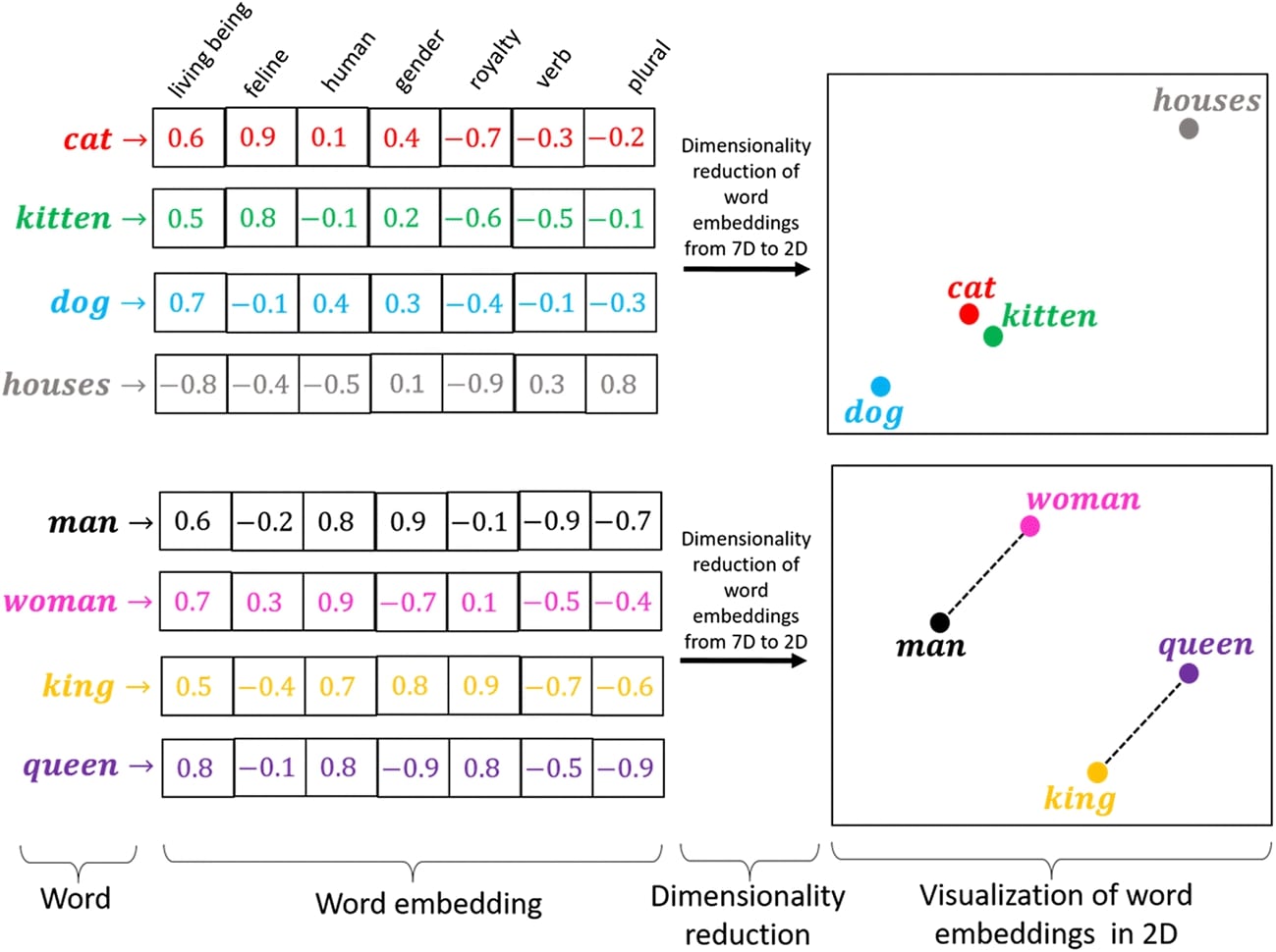
In this section, we are preparing our dataset so that it can be given to a neural network for training. We are going to use word embeddings approach to encoding text data. In order to encode data using this approach, we'll be following the below steps.
- Loop through each text example of data, Tokenize them and build a vocabulary of all unique tokens (words) from the corpus. The vocabulary is simply the mapping of tokens to a unique integer index. Each token is assigned a unique integer index starting from 0.
- Tokenize each text example to generate a list of tokens and then retrieve the index for each token from the vocabulary.
- Retrieve embeddings (real-valued vector) for each token index.
The first two steps will be completed in this section. The third step will be implemented in the neural network as an embedding layer which will be responsible for retrieving embeddings (real-valued vectors) for indexes.
Below, we have included a sample image showing the word embeddings concept.
1.1 Load Dataset
In this section, we have loaded the dataset that we are going to use for our text classification task. We have loaded AG NEWS dataset available from torchtext. The dataset has text documents for 4 different news categories (["World", "Sports", "Business", "Sci/Tech"]). The dataset is already divided into train and test sets. After loading them as normal arrays, we have wrapped them in ArrayDataset which is a commonly used wrapper in MXNet to maintain datasets.
from mxnet.gluon.data import ArrayDataset

train_dataset, test_dataset = torchtext.datasets.AG_NEWS()

Y_train, X_train = zip(*list(train_dataset))
Y_test,  X_test  = zip(*list(test_dataset))

train_dataset = ArrayDataset(X_train, Y_train)
test_dataset  = ArrayDataset(X_test, Y_test)
1.2 Define Tokenizer
In this section, we have defined a tokenizer for our task. A tokenizer is a function that takes a text document as input and returns a list of tokens as output. The tokens are generally words. We have created a tokenizer using regular expression. The expression splits a text document into a list of words.
import re
from functools import partial

tokenizer = partial(lambda X: re.findall(r"\w+", X))

tokenizer("Hello, How are you?")
1.3 Build Vocabulary
In this section, we have built a vocabulary of all unique tokens from our datasets. In order to build vocabulary, we need to provide a dictionary with all tokens and their respective frequencies in the dataset to Vocab() constructor available from gluonnlp. To create a dictionary of all tokens, we have first initialized Counter object from Python collections library. Then, we have looped through all text examples of datasets one by one calling count_tokens() method. We have provided the method with a list of tokens of text example and Counter object. The method updates tokens of text example in Counter object if they are not present there already.
Once, we loop through all text examples of the dataset, we have the Counter object ready with all unique tokens and their frequencies. We can then give this object to Vocab() constructor to create a vocabulary. We have printed the number of tokens of vocabulary as well at the end.
from collections import Counter

counter = Counter()

for dataset in [train_dataset, test_dataset]:
    for X, Y in dataset:
        gluonnlp.data.count_tokens(tokenizer(X), to_lower=True, counter=counter)

vocab = gluonnlp.Vocab(counter=counter, special_token="<unk>", min_freq=1)

print("Vocabulary Size : {}".format(len(vocab)))
1.4 Define Vectorization Function
In this section, we have defined the vectorization function which will be used by the data loaders we are going to create in the next section to map text documents to their respective token indexes using vocabulary.
The function takes as input a single batch of data which consists of a list of text examples and their respective target labels. It tokenizes each text example and retrieves token indexes for each of them. The number of tokens per text example can be of different lengths. In our case, we have decided to keep maximum of 50 tokens per text example. The text examples that have more than 50 tokens will be truncated to 50 tokens and text example that has less than 50 tokens will be padded with 0s to bring them to 50 tokens. In the end, MXNet Ndarrays consisting of token indexes and target labels will be returned from the vectorization function.
We have also explained how the function will work with one simple example.
import gluonnlp.data.batchify as bf
from mxnet import nd
import numpy as np

max_tokens = 50

clip_seq = gluonnlp.data.ClipSequence(max_tokens)
pad_seq  = gluonnlp.data.PadSequence(length=max_tokens, pad_val=0, clip=True)

def vectorize(batch):
    X, Y = list(zip(*batch))
    X = [[vocab(word) for word in tokenizer(sample)] for sample in X]
    #X = [sample+([0]* (max_tokens-len(sample))) if len(sample)<max_tokens else sample[:max_tokens] for sample in X] ## Bringing all samples to max_tokens length.
    X = [pad_seq(tokens) for tokens in X] ## Bringing all samples to 50 length
    return nd.array(X, dtype=np.int32), nd.array(Y, dtype=np.int32) - 1 # Subtracting 1 from labels to bring them in range 0-3 from 1-4

vectorize([["how are you", 1]])
1.5 Create Data Loaders
In this section, we have simply defined data loaders (train and test) using datasets. These data loaders will be used during the training process to loop through data in batches. The batch size is kept at 1024 text examples per batch. We have also provided the vectorization function defined in the previous section to batchify_fn parameter which will be applied to each batch of data.
from mxnet.gluon.data import DataLoader

train_loader = DataLoader(train_dataset, batch_size=1024, batchify_fn=vectorize)
test_loader  = DataLoader(test_dataset,  batch_size=1024, batchify_fn=vectorize)

target_classes = ["World", "Sports", "Business", "Sci/Tech"]
for X, Y in train_loader:
    print(X.shape, Y.shape)
    break
Approach 1: Single Conv1D Layer (Max Tokens=50, Embedding Length=128, Conv Output Channels=32) 
Our first approach uses CNN with a single 1D convolution layer for the text classification tasks. The network consists of three layers in total. The embedding layer, convolution layer, and dense layer. The embedding layer is responsible for mapping token indexes to their respective embeddings, the convolution layer performs convolution operation on the output of the embedding layer and the output of the convolution layer is given to the dense layer for generating 4 outputs (4 target categories) per text example.
Define Convolutional Neural Network
In this section, we have defined the network that we'll be using for our text classification task. The network consists of 3 layers.
- Embedding Layer
- Conv1D Layer
- Dense Layer
The embedding layer is the first layer of the network. We have created it using Embedding() constructor available from 'nn' sub-module of 'gluon' sub-module of MXNet*. We have provided the constructor with a length of vocabulary and embedding length. We have kept the embedding length at 128. This will create a weight matrix of shape (vocab_len, embed_len). When we call this layer with a list of indexes, it'll retrieve embeddings for those indexes from this weight matrix. The input to embedding layer will be of shape (batch_size, max_tokens) = (batch_size, 50) and output will be of shape (batch_size, max_tokens, embed_len) = (batch_size, 50, 128).
The output of embedding layer is reshape from shape (batch_size, max_tokens, embed_len) to shape (batch_size, embed_len, max_tokens). The reason behind doing this reshaping is that the convolution layer requires the channels dimension after the batch dimension and we want to treat the embedding dimension as the channels dimension hence we have moved it after the batch dimension.
The second layer of network is 1D convolution (Conv1D) layer. The layer is created with 32 output channels and kernel size of 7. This layer will translate input of shape (batch_size, embed_len, max_tokens) to (batch_size, conv_out_channels, max_tokens) = (batch_size, 32, 50). After applying convolution operation, it also applies relu activation to it.
On the output of convolution layer, we have called max() function at max tokens axis. This will transform shape from (batch_size, conv_out_channels, max_tokens) to (batch_size, conv_out_channels). Though we have used max() operation here, the reader can try other operations like min(), mean(), etc to see if they gives better results.
The output of this operation is given to Dense layer which has 4 output units. It transforms data from shape (batch_size, 32) to (batch_size, 4). The output of the dense layer is the prediction of the network.
After defining the network, we initialized it and performed a forward pass through it using random data for verification purposes. We have also printed the summary of network layers and their parameter count.
Please make a NOTE that we have not covered details of network creation in-depth. If you are someone new to MXNet library and want to learn how to create networks using it then we recommend that you go through the below links. They will help you get started designing neural networks using MXNet.
from mxnet.gluon import nn

embed_len = 128

class Conv1DTextClassifier(nn.Block):
    def __init__(self, **kwargs):
        super(Conv1DTextClassifier, self).__init__(**kwargs)
        self.word_embeddings = nn.Embedding(len(vocab), embed_len)
        self.conv1 = nn.Conv1D(channels=32, kernel_size=(7,), activation="relu", padding=(3,)) ## By default "NCW" is layout for CPU. On GPU, both "NCW" and "NWC" are supported
        self.linear1 = nn.Dense(len(target_classes))

    def forward(self, x):
        x = self.word_embeddings(x)
        x = x.reshape(len(x), embed_len, max_tokens) ## Embedding Length needs to be treated as channel dimension

        x = self.conv1(x)
        x = x.max(axis=-1) ## Taking max at output channels level. Hence we'll have one max value per output channel.

        logits = self.linear1(x)
        return logits #nd.softmax(logits)

model = Conv1DTextClassifier()

model
from mxnet import init, initializer

model.initialize(initializer.Xavier())

preds = model(nd.random.randint(1,len(vocab), shape=(10,50)))

preds.shape
model.summary(nd.random.randint(1,len(vocab), shape=(10,50)))
Train Network
In this section, we are training the network we defined earlier. To train the network, we have defined a function. The function takes a trained object (network parameters), train data loader, validation data loader, and a number of epochs as input. It then executes a training loop number of epochs time. During each epoch, it loops through whole training data in batches using a train data loader. For each epoch, the function performs a forward pass to make predictions, calculates loss, calculates gradients, and updates network parameters. The function records loss for each batch and prints the average loss per epoch at the end of an epoch. We have also created a helper function for calculating validation accuracy and loss values.
from mxnet import autograd
from tqdm import tqdm
from sklearn.metrics import accuracy_score

def MakePredictions(model, val_loader):
    Y_actuals, Y_preds = [], []
    for X_batch, Y_batch in val_loader:
        preds = model(X_batch)
        preds = nd.softmax(preds)
        Y_actuals.append(Y_batch)
        Y_preds.append(preds.argmax(axis=-1))

    Y_actuals, Y_preds = nd.concatenate(Y_actuals), nd.concatenate(Y_preds)
    return Y_actuals, Y_preds

def CalcValLoss(model, val_loader):
    losses = []
    for X_batch, Y_batch in val_loader:
        val_loss = loss_func(model(X_batch), Y_batch)
        val_loss = val_loss.mean().asscalar()
        losses.append(val_loss)
    print("Valid CrossEntropyLoss : {:.3f}".format(np.array(losses).mean()))

def TrainModelInBatches(trainer, train_loader, val_loader, epochs):
    for i in range(1, epochs+1):
        losses = [] ## Record loss of each batch
        for X_batch, Y_batch in tqdm(train_loader):
            with autograd.record():
                preds = model(X_batch) ## Forward pass to make predictions
                train_loss = loss_func(preds.squeeze(), Y_batch) ## Calculate Loss
            train_loss.backward() ## Calculate Gradients

            train_loss = train_loss.mean().asscalar()
            losses.append(train_loss)

            trainer.step(len(X_batch)) ## Update weights

        print("Train CrossEntropyLoss : {:.3f}".format(np.array(losses).mean()))
        CalcValLoss(model, val_loader)
        Y_actuals, Y_preds = MakePredictions(model, val_loader)
        print("Valid Accuracy         : {:.3f}".format(accuracy_score(Y_actuals.asnumpy(), Y_preds.asnumpy())))
Below, we have actually trained our network using the training function defined in the previous cell. We have initialized a number of epochs to 15 and the learning rate to 0.001. Then, we have initialized the text classifier, cross entropy loss, Adam optimizer, and Trainer object. At last, we have called our training routine with the necessary parameters to perform training. We can notice from the loss and accuracy values getting printed after each epoch that our network is doing a good job.
from mxnet import gluon
from mxnet.gluon import loss
from mxnet import autograd
from mxnet import optimizer

epochs=15
learning_rate = 0.001

model = Conv1DTextClassifier()
model.initialize()
loss_func = loss.SoftmaxCrossEntropyLoss()
optimizer = optimizer.Adam(learning_rate=learning_rate)

trainer = gluon.Trainer(model.collect_params(), optimizer)

TrainModelInBatches(trainer, train_loader, test_loader, epochs)
Evaluate Network Performance
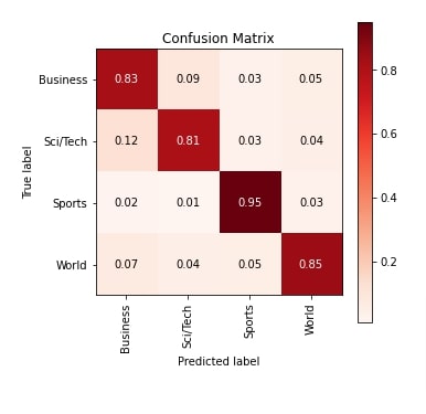
In this section, we have evaluated the performance of our trained network by calculating accuracy score, classification report and confusion matrix metrics on test predictions. We can notice from the accuracy score that our model is doing a good job at the text classification task, though it can be improved further. We have calculated all metrics using functions available from scikit-learn.
If you want to learn about various ML metrics available from sklearn then please check the below link which covers the majority of them in detail.
Apart from metrics calculation, we have also plotted the confusion matrix. From the plot, we can notice that our model is doing quite a good job at classifying text documents in Sports category compared to other target categories.
We have created a confusion matrix plot using Python library scikit-plot. It provides a charting facility for many ML metrics. Please feel free to check the below link if you want to learn about it.
from sklearn.metrics import accuracy_score, confusion_matrix, classification_report

Y_actuals, Y_preds = MakePredictions(model, test_loader)

print("Test Accuracy : {}".format(accuracy_score(Y_actuals.asnumpy(), Y_preds.asnumpy())))
print("Classification Report : ")
print(classification_report(Y_actuals.asnumpy(), Y_preds.asnumpy(), target_names=target_classes))
print("\nConfusion Matrix : ")
print(confusion_matrix(Y_actuals.asnumpy(), Y_preds.asnumpy()))
from sklearn.metrics import confusion_matrix
import scikitplot as skplt
import matplotlib.pyplot as plt
import numpy as np

skplt.metrics.plot_confusion_matrix([target_classes[i] for i in Y_actuals.asnumpy()], [target_classes[i] for i in Y_preds.asnumpy().astype(int)],
                                    normalize=True,
                                    title="Confusion Matrix",
                                    cmap="Reds",
                                    hide_zeros=True,
                                    figsize=(5,5)
                                    );
plt.xticks(rotation=90);
Explain Network Predictions Using LIME Algorithm
In this section, we have tried to explain network predictions using LIME algorithm. The python library lime provides an implementation of an algorithm. It let us create a visualization that highlights important words in the text document that contribute to predicting a particular target label.
If you are new to the concept of LIME and want to learn about it in depth then we recommend that you go through the below links in your free time as it'll help you enhance your knowledge of it.
- How to Use LIME to Understand sklearn Models Predictions?
- LIME: Interpret Predictions Of Keras Text Classification Networks
Below, we have first retrieved test examples from the test dataset.
X_test, Y_test = [], []
for X, Y in test_dataset:
    X_test.append(X)
    Y_test.append(Y-1)
Below, we have first created an instance of LimeTextExplainer object. This object will be used later to create an explanation object explaining prediction.
Then, we have created a prediction function that takes a batch of text examples as input and returns their probabilities.
After defining a function, we randomly selected a text example from the test dataset and predicted its target label using our trained network. Our network correctly predicts the target label as Sci/Tech for the selected text example. Next, we'll create an explanation and visualization for this text example.
from lime import lime_text

explainer = lime_text.LimeTextExplainer(class_names=target_classes, verbose=True)

def make_predictions(X_batch_text):
    X_batch = [[vocab(word) for word in tokenizer(sample)] for sample in X_batch_text]
    X_batch = [pad_seq(tokens) for tokens in X_batch] ## Bringing all samples to 50 length
    logits = model(nd.array(X_batch, dtype=np.int32))
    preds = nd.softmax(logits)
    return preds.asnumpy()

rng = np.random.RandomState(124)
idx = rng.randint(1, len(X_test))

X_batch = [[vocab(word) for word in tokenizer(sample)] for sample in X_test[idx:idx+1]]
X_batch = [pad_seq(tokens) for tokens in X_batch] ## Bringing all samples to 50 length
preds = model(nd.array(X_batch)).argmax(axis=-1)

print("Actual :     ", target_classes[Y_test[idx]])
print("Prediction : ", target_classes[int(preds.asnumpy()[0])])
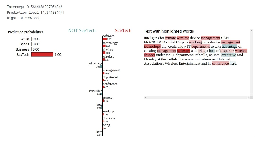
Below, we have first created an Explanation object by calling explain_instance() method on LimeTextExplainer object. We have provided selected a text example, a prediction function, and a target label. The explanation object has details about words contributing to prediction. Then, we have visualized the explanation object by calling show_in_notebook() method on it. We can notice from the visualization that words like 'software', 'technology', 'devices', 'wireless', 'management', 'departments', 'conference', etc are contributing to predicting target label as Sci/Tech.
explanation = explainer.explain_instance(X_test[idx], classifier_fn=make_predictions, labels=Y_test[idx:idx+1], num_features=15)
explanation.show_in_notebook()
Approach 2: Multiple Conv1D Layers (Max Tokens=50, Embedding Length=128, Conv Output Channels=[32,32]) 
Our approach in this section uses multiple convolution layers in CNN. The majority of code in this section is exactly the same as our previous section with only a change in network architecture where we are using two 1d convolution layers instead of one.
Define Network
Below, we have defined a network that we'll use for our classification task in this section. The network definition has one embedding layer, two convolution layers, and one dense layer. The input, as usual, is given to the embedding layer to generate embeddings which are given as input to the first convolution layer which has 32 output units, and applies kernel of shape 7 to input data. The max-pooling operation is applied to the output of the first convolution layer. The max pooled operation is given to the second convolution layer. We have then called max() function at the embedding dimension and given output to the dense layer. The output of the dense layer is a prediction of the network.
from mxnet.gluon import nn

embed_len = 128

class Conv1DTextClassifier(nn.Block):
    def __init__(self, **kwargs):
        super(Conv1DTextClassifier, self).__init__(**kwargs)
        self.word_embeddings = nn.Embedding(len(vocab), embed_len)

        self.conv1 = nn.Conv1D(channels=32, kernel_size=(7,), activation="relu", padding=(3,)) ## By default "NCW" is layout for CPU. On GPU, both "NCW" and "NWC" are supported
        self.max_pool = nn.MaxPool1D(pool_size=2) ## We can also try AvgPool
        self.conv2 = nn.Conv1D(channels=32, kernel_size=(7,), activation="relu", padding=(3,))

        self.linear1 = nn.Dense(len(target_classes))

    def forward(self, x):
        x = self.word_embeddings(x)
        x = x.reshape(len(x), embed_len, max_tokens) ## Embedding Length needs to be treated as channel dimension

        x = self.conv1(x)
        x = self.max_pool(x)
        x = self.conv2(x)

        x = x.max(axis=-1) ## Taking max at output channels level. Hence we'll have one max value per output channel.

        logits = self.linear1(x)
        return logits #nd.softmax(logits)

model = Conv1DTextClassifier()

model
from mxnet import init, initializer

model.initialize(initializer.Xavier())

preds = model(nd.random.randint(1,len(vocab), shape=(10,50)))

preds.shape
model.summary(nd.random.randint(1,len(vocab), shape=(10,50)))
Train Network
Below, we have trained our network using exactly the same settings that we had used earlier. We can notice from the loss and accuracy values getting printed after each epoch that our network is doing a good job at the text classification task.
from mxnet import gluon
from mxnet.gluon import loss
from mxnet import autograd
from mxnet import optimizer

epochs=15
learning_rate = 0.001

model = Conv1DTextClassifier()
model.initialize()
loss_func = loss.SoftmaxCrossEntropyLoss()
optimizer = optimizer.Adam(learning_rate=learning_rate)

trainer = gluon.Trainer(model.collect_params(), optimizer)

TrainModelInBatches(trainer, train_loader, test_loader, epochs)
Evaluate Network Performance
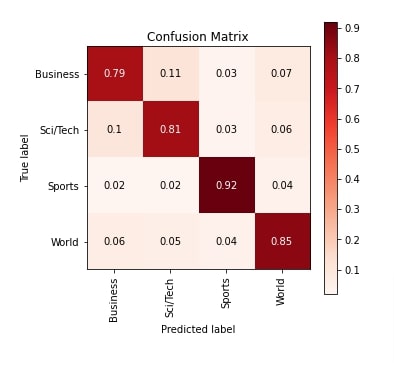
In this section, we have evaluated the performance of our trained network by calculating accuracy score, classification report and confusion matrix metrics on test predictions. We can notice from the accuracy score that it's a little less compared to our previous epoch which is surprising as we had expected more accuracy by lining more convolution layers. We have also plotted the confusion matrix for reference purposes.
from sklearn.metrics import accuracy_score, confusion_matrix, classification_report

Y_actuals, Y_preds = MakePredictions(model, test_loader)

print("Test Accuracy : {}".format(accuracy_score(Y_actuals.asnumpy(), Y_preds.asnumpy())))
print("Classification Report : ")
print(classification_report(Y_actuals.asnumpy(), Y_preds.asnumpy(), target_names=target_classes))
print("\nConfusion Matrix : ")
print(confusion_matrix(Y_actuals.asnumpy(), Y_preds.asnumpy()))
from sklearn.metrics import confusion_matrix
import scikitplot as skplt
import matplotlib.pyplot as plt
import numpy as np

skplt.metrics.plot_confusion_matrix([target_classes[i] for i in Y_actuals.asnumpy()], [target_classes[i] for i in Y_preds.asnumpy().astype(int)],
                                    normalize=True,
                                    title="Confusion Matrix",
                                    cmap="Reds",
                                    hide_zeros=True,
                                    figsize=(5,5)
                                    );
plt.xticks(rotation=90);
Explain Network Predictions Using LIME Algorithm
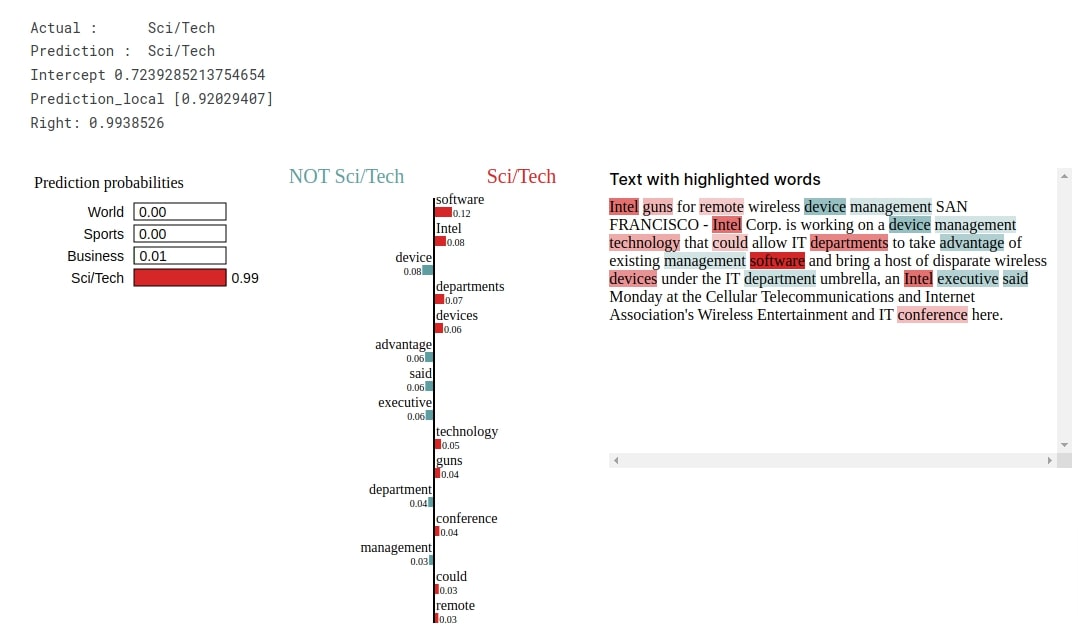
In this section, we have tried to explain predictions made by the trained network using LIME algorithm. The network correctly predicts the target label as Sci/Tech for the selected text example from the test dataset. The visualization highlights that words like 'software', 'intel', 'department', 'devices', 'technology', 'conference', 'remote', etc are used for predicting target label as Sci/Tech.
from lime import lime_text

explainer = lime_text.LimeTextExplainer(class_names=target_classes, verbose=True)

rng = np.random.RandomState(124)
idx = rng.randint(1, len(X_test))

X_batch = [[vocab(word) for word in tokenizer(sample)] for sample in X_test[idx:idx+1]]
X_batch = [pad_seq(tokens) for tokens in X_batch] ## Bringing all samples to 50 length
preds = model(nd.array(X_batch)).argmax(axis=-1)

print("Actual :     ", target_classes[Y_test[idx]])
print("Prediction : ", target_classes[int(preds.asnumpy()[0])])

explanation = explainer.explain_instance(X_test[idx], classifier_fn=make_predictions, labels=Y_test[idx:idx+1], num_features=15)
explanation.show_in_notebook()
4. Results Summary And Further Suggestions 
| Approach | Max Tokens | Embedding Length | Conv Output Channels | Test Accuracy (%) |
|---|---|---|---|---|
| Single Conv1D Layer Network | 50 | 128 | 32 | 86.03 |
| Multiple Conv1D Layers Network | 50 | 128 | 32,32 | 84.22 |
Further Recommendations
- Try different embedding lengths.
- Try different sizes of maximum tokens.
- Try different convolution layer output channels and kernel sizes.
- Try using average pooling between convolution layers.
- Try operation other than max() to the output of the convolution layer.
- Try different weight initialization methods.
- Train network for more epochs.
- Try using learning rate schedulers
This ends our small tutorial explaining how we can create CNNs with 1D convolution layers for text classification tasks using Python deep learning library MXNet. Please feel free to let us know your views in the comments section.
References
 Sunny Solanki
Sunny Solanki
Intro: Software Developer | Youtuber | Bonsai Enthusiast
About: Sunny Solanki holds a bachelor's degree in Information Technology (2006-2010) from L.D. College of Engineering. Post completion of his graduation, he has 8.5+ years of experience (2011-2019) in the IT Industry (TCS). His IT experience involves working on Python & Java Projects with US/Canada banking clients. Since 2020, he’s primarily concentrating on growing CoderzColumn.
His main areas of interest are AI, Machine Learning, Data Visualization, and Concurrent Programming. He has good hands-on with Python and its ecosystem libraries.
Apart from his tech life, he prefers reading biographies and autobiographies. And yes, he spends his leisure time taking care of his plants and a few pre-Bonsai trees.
Contact: sunny.2309@yahoo.in


![YouTube Subscribe]() Comfortable Learning through Video Tutorials?
Comfortable Learning through Video Tutorials?
If you are more comfortable learning through video tutorials then we would recommend that you subscribe to our YouTube channel.
![Need Help]() Stuck Somewhere? Need Help with Coding? Have Doubts About the Topic/Code?
Stuck Somewhere? Need Help with Coding? Have Doubts About the Topic/Code?
 Stuck Somewhere? Need Help with Coding? Have Doubts About the Topic/Code?
When going through coding examples, it's quite common to have doubts and errors.
If you have doubts about some code examples or are stuck somewhere when trying our code, send us an email at coderzcolumn07@gmail.com. We'll help you or point you in the direction where you can find a solution to your problem.
You can even send us a mail if you are trying something new and need guidance regarding coding. We'll try to respond as soon as possible.
![Share Views]() Want to Share Your Views? Have Any Suggestions?
Want to Share Your Views? Have Any Suggestions?
 Want to Share Your Views? Have Any Suggestions?
If you want to
- provide some suggestions on topic
- share your views
- include some details in tutorial
- suggest some new topics on which we should create tutorials/blogs
 mxnet, CNNs, 1d-convolutions, text-classification