Haiku (JAX): Simple Guide to Text Classification
Text classification is a supervised ML classification task where we classify text documents into categories. It has many applications like book classification, news article classification, spam mail classification, etc. Text is a type of unstructured data. In order to classify text documents, we first need to encode them. By encoding, we mean that we need to map text data to real-valued data as neural networks work with real-valued data. There are various strategies to encode text data (one-hot, word frequency, Tf-Idf, Word embeddings, etc).
As a part of this tutorial, we have explained how we can perform text classification through a neural network designed using Python deep learning library Haiku. Haiku is a high-level deep learning framework from DeepMind which is built on top of low-level framework JAX. Haiku was designed to simplify the task of network creation using JAX underneath. In order to encode text data, we'll use word frequency (bag of words) approach. The tutorial will get you started with handling text data. After training the network, we evaluated the performance by calculating various ML metrics. We have also explained predictions made by the network using LIME algorithm.
Below, we have listed important sections of our Tutorial to give an overview of the material covered.
Important Sections Of Tutorial
- Prepare Data
- 1.1 Load Data
- 1.2 Populate Vocabulary
- 1.3 Vectorize Data
- Define Network
- Define Loss Functions
- Train Network
- Evaluate Network Performance
- Explain Network Predictions using LIME Algorithms
Haiku Installation
- pip install -U dm-haiku
Below, we have imported the necessary Python libraries and printed the version that we have used in our tutorial.
import haiku as hk

print("Haiku Version :{}".format(hk.__version__))
import jax

print("JAX Version : {}".format(jax.__version__))
import optax

print("Optax Version : {}".format(optax.__version__))
from tensorflow import keras

print("Keras Version : {}".format(keras.__version__))
1. Prepare Data 
In this section, we are preparing data for the network. As mentioned earlier, we'll be encoding data using word frequency (bag of words) approach. In order to encode data and make it ready for the network, we'll follow the below steps.
- Load Data.
- Populate vocabulary of unique words present in all text docs. In order to populate vocabulary, we'll tokenize each text example. The tokenization will break the text example into a list of tokens (words). The vocabulary is a simple mapping from a word to an integer index. Each word is assigned a unique index starting from 0.
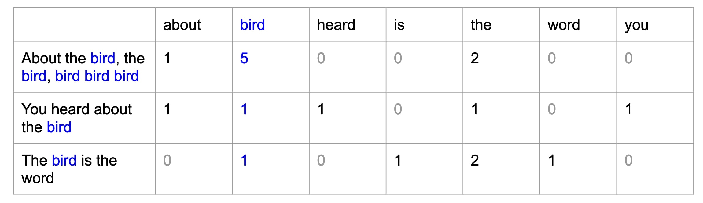
- Vectorize each text example. For each text example/document, a vector of length same as vocabulary length will be created. In that vector, the frequency of words will be present at their index location of vocabulary. As all vocabulary words won't be present in single text documents, the words which are not there will have a frequency of 0.
The vectorized data will be given to network for training purposes. Don't worry if you don't understand steps 100% as they will become clear once we go through them.
1.1 Load Data
Here, we are loading the newsgroups dataset available from scikit-learn. The dataset has text documents for 20 different news categories. We have selected 4 categories from those for our purpose. The dataset is already divided into train and test sets which we have loaded using fetch_20newsgroups().
import numpy as np
from sklearn import datasets
import gc

all_categories = ['alt.atheism','comp.graphics','comp.os.ms-windows.misc','comp.sys.ibm.pc.hardware',
                  'comp.sys.mac.hardware','comp.windows.x', 'misc.forsale','rec.autos','rec.motorcycles',
                  'rec.sport.baseball','rec.sport.hockey','sci.crypt','sci.electronics','sci.med',
                  'sci.space','soc.religion.christian','talk.politics.guns','talk.politics.mideast',
                  'talk.politics.misc','talk.religion.misc']

target_classes = ['comp.graphics','rec.autos','rec.sport.hockey', 'talk.religion.misc']

X_train_text, Y_train = datasets.fetch_20newsgroups(subset="train", categories=target_classes, return_X_y=True)
X_test_text , Y_test  = datasets.fetch_20newsgroups(subset="test", categories=target_classes, return_X_y=True)

classes = np.unique(Y_train)
mapping = dict(zip(classes, target_classes))

len(X_train_text), len(X_test_text), classes, mapping
1.2 Populate Vocabulary
Keras library provided Tokenizer object which will let us populate vocabulary as well as vectorize data. Here, we have first created Tokenizer object and called fit_on_texts() on object with train & test datasets. This method will populate vocabulary in the tokenizer object by tokenizing each text example from train and test datasets one by one. After populating vocabulary, we have also printed the length of vocabulary as well as a few mappings from it. The vocabulary is available through index_word property of the tokenizer object.
from keras.preprocessing.text import Tokenizer
from keras.preprocessing.sequence import pad_sequences
from jax import numpy as jnp

tokenizer = Tokenizer()
tokenizer.fit_on_texts(X_train_text+X_test_text)

print("Vocabulary Size : {}".format(len(tokenizer.index_word)))

print("Vocabulary Starts @ Index 1: {}".format(list(tokenizer.index_word.items())[:5]))
1.3 Vectorize Data
Here, we have vectorized our text data using a tokenizer object which has vocabulary present in it. In order to tokenize data, we have called texts_to_matrix() method on the tokenizer object with train and test datasets one by one. It'll return arrays that have vectorized data. The output shape of arrays are (train_examples, vocab_len) and (test_examples, vocab_len). After vectorizing data, we have also printed one example to show how it looks.
Below, we have included an image that shows the vectorization process. It'll help you better understand it.
X_train_vect = tokenizer.texts_to_matrix(X_train_text, "count")
X_test_vect  = tokenizer.texts_to_matrix(X_test_text, "count")

X_train_vect, X_test_vect = jnp.array(X_train_vect, dtype=jnp.float32), jnp.array(X_test_vect, dtype=jnp.float32)
Y_train, Y_test = jnp.array(Y_train), jnp.array(Y_test)

X_train_vect.shape, X_test_vect.shape
X_train_vect[1][:100]
print(X_train_text[1])
2. Define Network 
In this section, we have defined a network that we'll use for our text classification task. The network consists of 3 linear layers with output units 128, 64, and 4 respectively. Inside the forward pass method, we are applying relu activation to the output of the first and second linear layers. The output of the third linear layer is a prediction of our network.
After defining the network, we have transformed the class-based model to JAX pure function-based model and initialized it. After initializing, we have printed the shape of weights/biases of layers and also performed a forward pass for verification purposes.
Please make a NOTE that we have not covered how to design a network using Haiku in detail. Please feel free to check the below link if you are new to Haiku and want to learn how to create a network using it.
class TextClassifier(hk.Module):
    def __init__(self):
        super().__init__(name="TextClassifier")
        self.linear1 = hk.Linear(128, name="Dense1")
        self.linear2 = hk.Linear(64, name="Dense1")
        self.linear3 = hk.Linear(len(target_classes), name="Dense1")

    def __call__(self, X_batch):
        x = jax.nn.relu(self.linear1(X_batch))
        x = jax.nn.relu(self.linear2(x))

        return self.linear3(x)
def TextClassifierNet(x):
    classif = TextClassifier()
    return classif(x)

text_classif = hk.transform(TextClassifierNet)
rng = jax.random.PRNGKey(42)

params = text_classif.init(rng, X_train_vect[:5])

print("Weights Type : {}\n".format(type(params)))

for layer_name, weights in params.items():
    print(layer_name)
    print("Weights : {}, Biases : {}\n".format(params[layer_name]["w"].shape,params[layer_name]["b"].shape))
preds = text_classif.apply(params, rng, X_train_vect[:5])

preds[:5]
3. Define Loss Function 
In this section, we have defined a Cross entropy loss function that we'll be using for our task. The function takes network parameters, input data, and actual target values as input. It then performs a forward pass through the network using input data & parameters to make predictions and one-hot encodes actual target values. At last, it calculates loss using softmax_cross_entropy() function available from optax library and returns it. The optax is a Python library that provides many optimizers and loss functions for JAX related libraries.
def CrossEntropyLoss(params, input_data, actual):
    logits_preds = model.apply(params, rng, input_data)
    one_hot_actual = jax.nn.one_hot(actual, num_classes=len(target_classes))
    return optax.softmax_cross_entropy(logits=logits_preds, labels=one_hot_actual).sum()
4. Train Network 
In this section, we have trained our network. In order to train it, we have designed a simple helper function. The function takes train data (X_train, Y_train), validation data (X_val, Y_val), number of epochs, network parameters, optimizer state, and batch size as input. It executes a training loop number of epochs time. For each epoch, it loops through training data in batches. For each batch of data, it performs a forward pass to make predictions, calculates loss, calculates gradients, and updates network parameters using gradients. It records the loss of every batch and prints the average loss at the end of each epoch. We are also calculating validation accuracy at the end of each epoch to check network performance on validation data. The function at last returns updated network parameters.
from jax import value_and_grad
from tqdm import tqdm
from sklearn.metrics import accuracy_score

def TrainModelInBatches(X_train, Y_train, X_val, Y_val, epochs, params, optimizer_state, batch_size=32):
    for i in range(1, epochs+1):
        batches = jnp.arange((X_train.shape[0]//batch_size)+1) ### Batch Indices

        losses = [] ## Record loss of each batch
        for batch in tqdm(batches):
            if batch != batches[-1]:
                start, end = int(batch*batch_size), int(batch*batch_size+batch_size)
            else:
                start, end = int(batch*batch_size), None

            X_batch, Y_batch = X_train[start:end], Y_train[start:end] ## Single batch of data

            loss, gradients = value_and_grad(CrossEntropyLoss)(params, X_batch, Y_batch)

            #params = jax.tree_map(UpdateWeights, params, param_grads) ## Update Params
            updates, optimizer_state = optimizer.update(gradients, optimizer_state)
            params = optax.apply_updates(params, updates)
            losses.append(loss) ## Record Loss

        print("CrossEntropy Loss : {:.3f}".format(jnp.array(losses).mean()))
        gc.collect()
        Y_val_preds = model.apply(params, rng, X_val)
        val_acc = accuracy_score(Y_val, jnp.argmax(Y_val_preds, axis=1))
        print("Validation  Accuracy : {:.3f}".format(val_acc))
        gc.collect()
    return params
Below, we are actually training our network by calling the training function designed in the previous cell. We have initialized a number of epochs to 5, batch size to 32, and learning rate to 0.001. Then we initialized the network and Adam optimizer. At last, we have called our training routine with the necessary parameters to perform the training process. We can notice from the loss and accuracy values getting printed after each epoch that our network is doing a good job at the classification task.
from jax import value_and_grad

rng = jax.random.PRNGKey(42) ## Reproducibility ## Initializes model with same weights each time.
epochs = 5
batch_size = 32
learning_rate = 1e-3

model = hk.transform(TextClassifierNet)
params = model.init(rng, X_train_vect[:5])
optimizer = optax.adam(learning_rate=learning_rate)
optimizer_state = optimizer.init(params)

final_params = TrainModelInBatches(X_train_vect, Y_train, X_test_vect, Y_test, epochs, params, optimizer_state, batch_size=batch_size)
5. Evaluate Network Performance 
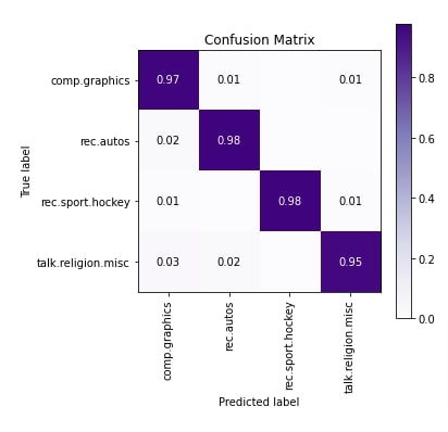
In this section, we have evaluated the performance of our trained network by calculating metrics like accuracy score, classification report (precision, recall, and f1-score per target class), and confusion matrix. We can notice from the accuracy score that our network is doing quite a good job. We have calculated these metrics using functions available from scikit-learn.
Please feel free to check the below link if you want to learn about various ML metrics available from sklearn.
Below these calculations, we have also plotted the confusion matrix to have a better look at the performance of our network for individual target classes. We can notice from the chart that our network is doing good for all 4 target categories. The chart is created using Python library scikit-plot.
Please feel free to check the below link if you want to learn about scikit-plot. It provides an implementation of many ML metrics.
from sklearn.metrics import accuracy_score, classification_report, confusion_matrix

train_preds = model.apply(final_params, rng, X_train_vect)
test_preds = model.apply(final_params, rng, X_test_vect)

print("Train Accuracy : {:.3f}".format(accuracy_score(Y_train, np.argmax(train_preds, axis=1))))
print("Test  Accuracy : {:.3f}".format(accuracy_score(Y_test, np.argmax(test_preds, axis=1))))
print("\nClassification Report : ")
print(classification_report(Y_test, np.argmax(test_preds, axis=1), target_names=target_classes))
print("\nConfusion Matrix : ")
print(confusion_matrix(Y_test, np.argmax(test_preds, axis=1)))
from sklearn.metrics import confusion_matrix
import scikitplot as skplt
import matplotlib.pyplot as plt

skplt.metrics.plot_confusion_matrix([target_classes[i] for i in Y_test], [target_classes[i] for i in np.argmax(test_preds, axis=1)],
                                    normalize=True,
                                    title="Confusion Matrix",
                                    cmap="Purples",
                                    hide_zeros=True,
                                    figsize=(5,5)
                                    );
plt.xticks(rotation=90);
6. Explain Network Predictions using LIME Algorithm 
In this section, we'll go a little further to check network performance. We'll interpret the results of prediction using LIME (Local Interpretable Model-Agnostic Explanations) algorithm. The algorithm let us understand which tokens (words) of text examples contributed to predicting a particular target category. This can be very helpful to interpret whether the network is using words that make sense to predict. We'll use the implementation of the algorithm available from the Python library lime. It let us visualize prediction showing which words contributed to prediction.
If you are someone who is new to the concept of LIME and want to learn about it in-depth then we recommend that you go through the below links. It'll help you greatly.
- How to Use LIME to Understand sklearn Models Predictions?
- LIME: Interpret Predictions Of Keras Text Classification Networks
In order to explain prediction using lime, we need to create an instance of Explainer first. Below, we have created an instance of LimeTextExplainer first.
from lime import lime_text

explainer = lime_text.LimeTextExplainer(class_names=target_classes, verbose=True)
Here, we have created a prediction function. The function takes a list of text examples as input and returns predictions made on them by our network. It tokenizes and vectorizes data before giving it to the network for prediction. This function will be used by the lime explainer object.
After defining a function, we randomly selected a text example from the test dataset and made a prediction on that. We can notice that our network is correctly predicting the target category as 'rec.sport.hockey' for the selected text example. Next, we'll create an explanation object explaining this prediction and visualize it.
import numpy as np

def make_predictions(X_batch_text):
    X_batch = tokenizer.texts_to_matrix(X_batch_text, "count")
    preds = model.apply(final_params, rng, jnp.array(X_batch))
    preds = jax.nn.softmax(preds)
    return preds.to_py()

rnd_st = np.random.RandomState(3)
idx = rnd_st.randint(1, len(X_test_text))

print("Prediction : ", target_classes[model.apply(final_params, rng, X_test_vect[idx:idx+1]).argmax(axis=-1)[0]])
print("Actual :     ", target_classes[Y_test[idx]])
Below, we have first called explain_instance() method on the explainer object to create an Explanation instance. We have provided a text example, prediction function, and target value to the function.
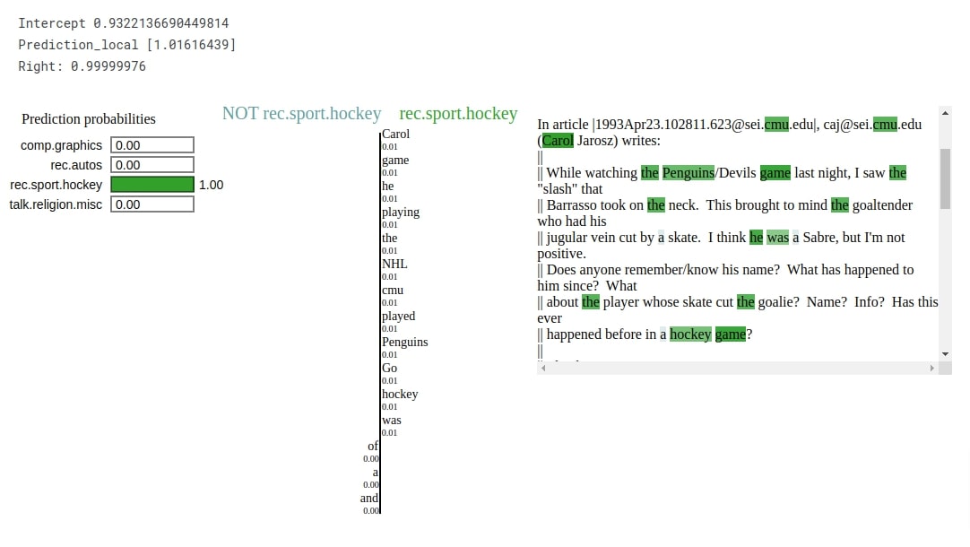
Then, we have called show_in_notebook() method on the explanation instance to create a visualization showing the contribution of words towards predicting the target label as 'rec.sport.hockey'.
We can notice from the visualization that words like 'game', 'playing', 'he', 'hockey', 'penguins', 'NHL', etc are used for predicting target label as 'rec.sport.hockey'. This makes sense as these are commonly used words in the hockey world.
explanation = explainer.explain_instance(X_test_text[idx], classifier_fn=make_predictions, labels=Y_test[idx:idx+1].to_py(), num_features=15)
explanation.show_in_notebook()
 Sunny Solanki
Sunny Solanki
Intro: Software Developer | Youtuber | Bonsai Enthusiast
About: Sunny Solanki holds a bachelor's degree in Information Technology (2006-2010) from L.D. College of Engineering. Post completion of his graduation, he has 8.5+ years of experience (2011-2019) in the IT Industry (TCS). His IT experience involves working on Python & Java Projects with US/Canada banking clients. Since 2020, he’s primarily concentrating on growing CoderzColumn.
His main areas of interest are AI, Machine Learning, Data Visualization, and Concurrent Programming. He has good hands-on with Python and its ecosystem libraries.
Apart from his tech life, he prefers reading biographies and autobiographies. And yes, he spends his leisure time taking care of his plants and a few pre-Bonsai trees.
Contact: sunny.2309@yahoo.in


![YouTube Subscribe]() Comfortable Learning through Video Tutorials?
Comfortable Learning through Video Tutorials?
If you are more comfortable learning through video tutorials then we would recommend that you subscribe to our YouTube channel.
![Need Help]() Stuck Somewhere? Need Help with Coding? Have Doubts About the Topic/Code?
Stuck Somewhere? Need Help with Coding? Have Doubts About the Topic/Code?
 Stuck Somewhere? Need Help with Coding? Have Doubts About the Topic/Code?
When going through coding examples, it's quite common to have doubts and errors.
If you have doubts about some code examples or are stuck somewhere when trying our code, send us an email at coderzcolumn07@gmail.com. We'll help you or point you in the direction where you can find a solution to your problem.
You can even send us a mail if you are trying something new and need guidance regarding coding. We'll try to respond as soon as possible.
![Share Views]() Want to Share Your Views? Have Any Suggestions?
Want to Share Your Views? Have Any Suggestions?
 Want to Share Your Views? Have Any Suggestions?
If you want to
- provide some suggestions on topic
- share your views
- include some details in tutorial
- suggest some new topics on which we should create tutorials/blogs
 haiku, jax, text-classification