Simple Guide to Text Classification Using MXNet¶

Text classification task also sometimes referred to as document classification is a task of classifying text documents into particular categories based on their texts. We generally encounter these kinds of tasks like classifying books at a library, classifying news articles, classifying blogs, classifying forum comments, etc. We can design a deep neural network to perform text classification tasks but we need to encode text data first as neural networks require input to be real-value and not text. There are various ways to encode text data like word frequency, Tf-Idf, one-hot encoding, word embeddings, etc.

In this tutorial, we have explained how we can perform text classification tasks using Python MXNet deep learning library. We have used various functions from gluonnlp library when encoding text examples. We have used the newsgroup dataset available from scikit-learn and encoded texts using word frequency approach. Then, we have performed classification by designing a neural network. We have also evaluated the performance of the network by calculating various ML metrics and explained network predictions using LIME algorithm and SHAP Values.

Below, we have listed important sections of tutorial to give an overview of the material covered.

Important Sections Of Tutorial¶

1. Prepare Data
   • 1.1 Load Dataset
   • 1.2 Define Tokenizer
   • 1.3 Populate Vocabulary
   • 1.4 Define Vectorization Function
   • 1.5 Define Data Loaders
2. Define Network
3. Train Network
4. Evaluate Network Performance
5. Explain Predictions Using LIME Algorithm
6. Explain Network Predictions Using SHAP Values

Below, we have loaded libraries and printed the versions that we have used in our tutorial.

1. Prepare Data ¶

In this section, we have prepared our dataset so that it can be given directly to the neural network for training purposes. The steps taken to prepare data include a loading of text datasets, tokenizing data examples, populating vocabulary with tokens of examples, and creating data loaders that load batches of vectorized data examples. We'll be using the word frequency approach to vectorize our data hence we'll record the frequency of tokens per text document and give it as input to the network.

1.1 Load Dataset¶

In this section, we have loaded the newsgroups dataset that we'll be using for our text classification task. It is available from datasets sub-module of scikit-learn. The dataset has text documents for 20 different news categories. We have selected 5 news categories for our purpose. After loading train and test examples, we have created ArrayDataset object using them which will be given to creating data loader objects later.

1.2 Define Tokenizer¶

In this section, we have created a tokenizer that we'll use to tokenize our text example. Our approach to encoding text data to real-value data consists of first tokenizing text documents and then calculating the frequency of tokens per text document. Below, we have created a simple function using regular expression that captures one or more subsequent characters and counts them as a token. We have used partial() function from functools Python library to create tokenization function.

We have also called the tokenization function on sample text to show how it generates a list of tokens from given input text.

1.3 Populate Vocabulary¶

In this section, we have populated a vocabulary that will be later used for the encoding of tokens. A vocabulary is a simple dictionary that has a mapping from a token to a unique integer index. Each token is assigned a unique integer index starting from integer 0.

In order to create a vocabulary, we first need to get a list of all tokens from all text examples. To do that, we are looping through our datasets (train and test) and all text examples of those datasets calling count_tokens() function from data sub-module of gluonnlp library each time. This function takes a list of tokens and Counter object as input. It keeps on updating Counter objects with tokens and their frequencies. We have initially created an empty Counter object, to begin with. After both loops have been completed, the counter object will have all possible tokens and their frequencies in it. The Counter object is a simple dictionary available from collections module that takes as an input list of items and creates a dictionary where keys are items and values are their frequencies in the input list. Please check the below link if you want to know about Counter in detail.

• Collections In Python

After populating Counter object, we have created a vocabulary by calling Vocab() constructor from gluonnlp with Counter object. We have set min_freq to 1 to inform the constructor to keep only tokens that appear at least once. We have also printed the size of the vocabulary at last.

1.4 Define Vectorization Function¶

In this section, we have defined a simple function that will be used to vectorize text data. We'll be using CountVecorizer available from scikit-learn to vectorize text data. We have initialized CountVectorizer using our vocabulary and tokenizer. The vectorizer simply takes a text example as input and returns a vector (of the same length as vocabulary size) which has a frequency of tokens present at the index of that token in vocabulary. To explain it with a simple example, let's say, we have a simple vocabulary of 8 words and we want to encode the text example given below.

text = "Hello, How are you? Where are you planning to go?"

vocab = {
    'hello': 0,
    'bye': 1,
    'how': 2,
    'the': 3,
    'welcome': 4,
    'are': 5,
    'you': 6,
    'to': 7
}

vector = [1, 0, 1, 0, 0, 2, 2, 1]

We can notice from the vector above that the frequency of tokens is present at an index of those tokens as per vocabulary. For example, the 5th index which is an index of 'are' token has a frequency count of 2 because it appears two times in the text example.

Please feel free to check the below tutorial if you want to learn about CountVectorizer and the various functionalities it provides in detail.

• Scikit-Learn - Feature Extraction from Text Data

Our vectorizer function takes as an input batch of data that has a list of text examples and their respective target labels. It then vectorizes text examples using a count vectorizer and returns vectorized examples and their target labels. It converts data to mxnet ndarray before returning. We have also explained with one simple example how the vectorization function works.

1.5 Define Data Loaders¶

In this section, we have created data loaders (train and test) using datasets we created earlier. These data loaders will be used during the training process to loop through data in batches. We have set the batch size to 1024 which means one batch will have that many examples. We have also provided our vectorization function from the previous section to batchify_fn parameter which will put batch data through it to return vectorized data which can be given directly to the neural network.

2. Define Network ¶

In this section, we have created a neural network that we'll use for our text classification task. The network consists of three dense layers with output units 128, 64, and 5 (no of target classes) respectively. The first two dense layers have relu as the activation function. We have created a network using Sequential API of mxnet. Please feel free to check the below link if you are new to MXNet and want to learn how to create a neural network using it.

• MXNet: Guide to Create Neural Networks

After defining the network, we initialized it and performed a forward pass with random data for verification purposes.

3. Train Network ¶

Here, we have trained our network. To train it, we have defined a simple function that takes the trainer object, train data loader, validation data loader, and a number of epochs as input to perform training. It then executes a training loop number of epochs time. For each epoch, it loops through training data in batches using a train data loader. For each batch of data, it performs a forward pass to make predictions, calculate loss, calculate gradients, and update network parameters. It also prints the average loss of all batches at the end of each epoch. We have also created two other helper functions that can be used to calculate validation loss and validation accuracy.

Below, we have actually performed training using a function defined in the previous cell. We have initialized a number of epochs to 8 and the learning rate to 0.001. Then, we have initialized our text classification network, cross entropy loss, Adam optimizer, and Trainer object. At last, we have called our training routine to perform training. We can notice from the loss and accuracy getting printed after each epoch that our model is doing quite a good job at classifying text documents.

4. Evaluate Network Performance ¶

In this section, we have evaluated the performance of the network by calculating accuracy, classification report (precision, recall, and f1-score) and confusion matrix metrics on test predictions. We can notice from the accuracy score that our model has done a decent job at the task. We have calculated all the ML metrics using functions available from scikit-learn. Please feel free to check the below link if you want to learn about various ML metrics available from sklearn.

• Scikit-Learn - Model Evaluation & Scoring Metrics

We have also created the plot of the confusion matrix using scikit-plot library. The plot helps us better understand which categories our model is doing good and for which worse. Except, 'talk.politics.misc' category, our model is doing a good job in all other categories. Please feel free to check the below link if you want to learn about various ML metrics plots available from scikit-plot.

• Scikit-Plot: Visualizing Machine Learning Algorithm Results & Performance Metrics

5. Explain Predictions Using LIME Algorithm ¶

In this section, we have explained predictions made by our network using LIME algorithm. It is a commonly used algorithm to explain the predictions of black-box ML algorithms. We'll be using lime python library to create an explanation of prediction. It creates a visualization highlighting words that contributed to predicting a particular target label.

In order to create an explanation using LIME, we need to follow a list of steps that we have followed next. Please feel free to go through the below tutorials if you are new to LIME algorithm and want to know in-depth about it.

• How to Use LIME to Understand sklearn Models Predictions?
• LIME: Interpret Predictions Of Keras Text Classification Networks

5.1 Create Explainer¶

In this section, we have first created an instance of LimeTextExplainer. This instance will be used to generate Explanation object later by calling explain_instance() method on it which will have details about words contributing to predicting the target label.

5.2 Select Random Text Example And Make Prediction¶

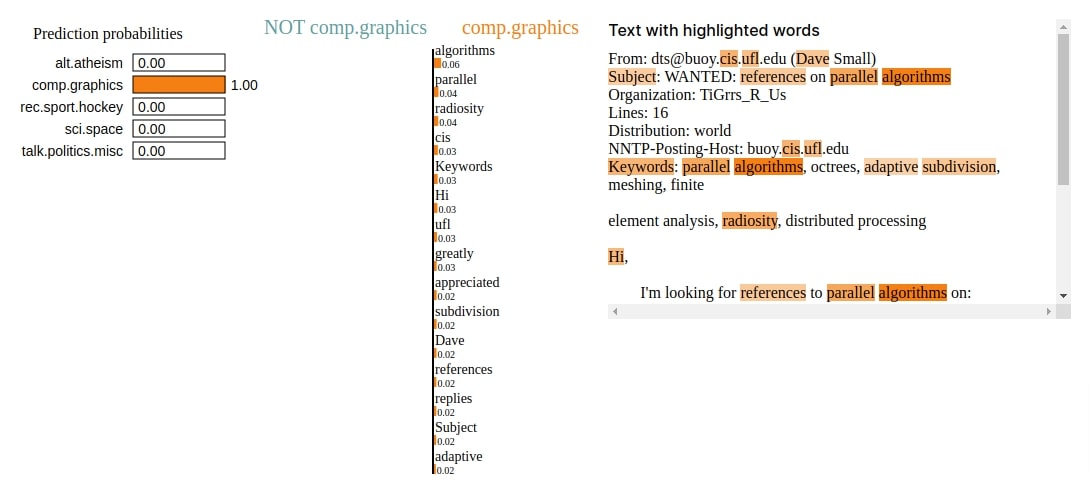
In this section, we have simply randomly selected a text example from the test set and made predictions on it using our trained model. Our model correctly predicts the target category as 'comp.graphics' for the selected text example.

5.3 Create Explanation For Selected Text Example And Visualize Explanation¶

In this section, we have created an explanation visualization that shows words contributing to prediction. We have first created a simple prediction function that takes a batch of text examples as input and returns their probabilities using our trained model. It vectorizes the input text examples and gives them to model to return predictions. It then applies softmax function on network output to generate probabilities and return them.

After defining the function, we have called explain_instance() method with selected text example, prediction function, and actual target label as input. It returns an Explanation object. We have then called show_in_notebook() method on Explanation object to generate visualization explaining prediction category 'comp.graphics'. We can notice from the visualization that words like 'algorithms', 'parallel', 'radiosity', 'adaptive', 'references', etc are contributing to predicting category as 'comp.graphics' which makes sense as these are commonly used word in the computer graphics field.

6. Explain Network Predictions Using SHAP Values ¶

In this section, we have explained the predictions made by our network by generating SHAP values and visualizing them. We have followed a series of steps to generate the visualizations below.

Please feel free to go through the below tutorials if you are new to SHAP values as it'll help you get started with it and also give you detailed knowledge about it.

• SHAP - Explain Machine Learning Model Predictions using Game Theoretic Approach
• Explain Text Classification Models Using SHAP Values (Keras + Vectorized Data)

6.1 Define Predictions Function, Masker, and Explainer¶

In order to generate SHAP values, we need to create an Explainer object first. We need to give masker and prediction function to explainer object. We have defined a simple prediction function below that takes a batch of text examples as input and returns their predicted probabilities by our trained model. The masker is simple regular expression that is used to hide parts of text not contributing to predictions (spaces generally).

After defining the prediction function and masker, we have created Explainer object using them.

6.2 Generate SHAP Values For Selected Samples¶

Here, we have simply selected two text examples from our test set and made predictions on them using our trained network. Our network correctly predicts target labels as 'sci.space' and 'talk.politics.misc' for selected examples. We have also printed the probabilities of predictions.

After making predictions, we have generated SHAP values by calling the explainer object with two text examples. In the next sections, we'll visualize these values.

6.3 Text Plot¶

Below, we have generated text plot by calling text_plot() method with SHAP values. It generates a visualization with original text of examples and highlights words contributing negatively/positively to predicting target labels. We can notice from the visualization that for first example, words like 'sky', 'space', 'high-speed', 'collision', 'sun', 'temperature', etc are contributing to predicting target label as 'sci.space' and for second example, words like 'republican', 'administration', 'reliance', 'organization', 'tear gas', 'govt', 'taxes', etc are contributing to predicting target label as 'talk.politics.misc'.

6.4 Bar Plots¶

Below, we have generated a bar chart of word grouping contributing to the prediction of the first text example and then in the next cell, we have created a bar chart for the second text example.

This ends our small tutorial explaining how we can perform text classification using MXNet. Please feel free to let us know your views in the comments section.

References¶

• MXNet: Guide to Create Neural Networks
• How to use Word Embeddings with MXNet for Text Classification?