Scikit-Optimize: Simple Guide to Hyperparameters Tunning / Optimization¶

What is Hyperparameters Tuning / Optimization?¶

Hyperparameters optimization is a process where we find values of hyperparameters of the ML model that gives the best results in less time without trying all possible combinations.

ML models for complicated problems generally have lots of hyperparameters and trying all possible combinations (grid search) of those hyperparameters' values on a large amount of data can take a lot of time even on modern computers.

We need an efficient way of finding values of hyperparameters in less amount of time that gives the best results so that we can try more experiments.

Which Python Libraries Can Perform Hyperparameters Tuning?¶

Python has many libraries for Machine Learning (scikit-learn, statsmodels, xgboost, lightgbm, catbooxt, keras, PyTorch, JAX, MXNet, etc). Python has libraries for tuning hyperparameters of ML Models created using these libraries as well (optuna, scikit-optimize, hyperopt, bayes_opt, sklearn-grid search, keras-tuner, etc).

What Can You Learn From This Article?¶

As a part of this tutorial, we have explained how to perform hyperparameters tuning of sklearn ML Models using Python library scikit-optimize with simple and easy-to-understand examples. Tutorial covers how to perform hyperparameters tuning for regression and classification models. Tutorial also covers plotting functionality available from scikit-optimize. Tutorial is a good starting point for someone who is new to scikit-optimize.

Scikit-optimize performs bayesian optimization using a gaussian process to find the best hyperparameters settings that minimize objective / loss value as much as possible. It finds optimal settings in less amount of time as well. It let us minimize the output value of almost any black-box function.

Below, we have listed important sections of Tutorial to give an overview of the material covered.

Important Sections Of Tutorial¶

1. Steps to Use Scikit-Optimize
2. Minimize Simple Line Formula
   • Define Objective Function
   • Define HyperParameters Search Space
   • Minimize Objective Function
   • Print Results
   • Minimize over Float Search Space
   • Define Search Space using "skopt.space" Module
3. Hyperparameters Tuning of Scikit-Learn Regression Model
   • Load Dataset
   • Define Hyperparameters Search Space
   • Define Objective Function
   • Optimize Objective Function (Minimize for Least MSE)
   • Print Best Results
   • Train and Evaluate Model with Best Hyperparameters
4. Hyperparameters Tuning of Scikit-Learn Classification Model
   • Same sub-sections as Regression (except we Maximize for Accuracy)
5. Plotting to Understand Tuning Process Results
   • Gaussian Process and Optimization Results for 1D Objective Functions
   • Partial Dependence Plots of Objective Function
   • Partial Dependence Plot of 2 Hyperparameters Combination
   • Hyperparameters Search Space Sampling Plot
   • Hyperparameter Search Space Sampling Histogram
   • Convergence Plot
   • Cumulative Regret Plot

We'll start by importing the necessary Python libraries.

1. Steps to Use Scikit-Optimize for Hyperparameters Tuning ¶

1. Define an Objective Function.
   • This is the step where we declare a function that takes a single combination of hyperparameters as input, creates a model, trains it, and evaluates it. We return some metric value (MSE, MAE, log loss, etc.) at the end of the function which we want to minimize.
2. Define Hyperparameters Search Space.
   • This is the step where we declare a list of hyperparameters that we want to optimize and the range of values of those hyperparameters to try.
3. Minimize Objective function value by trying different hyperparameters combinations using the bayesian process.
   • This is the step where scikit-optimize will try different combinations of hyperparameters settings on the objective function and try to minimize the output metric value in less amount of time.

We'll first try to explain the usage of scikit-optimize by minimizing the output value of the simple line formula following the steps mentioned above. It's a kind of optional section that you can skip if you are in hurry and want to learn how to use scikit-optimize with skearn models directly.

We'll then explain how we can use a library with scikit-learn models. We'll also explore plotting functionality available through scikit-optimize.

2. Minimize Simple Line Formula ¶

NOTE: Please feel free to skip this section if you are in hurry and want to learn how to use "scikit-optimize" with Scikit-learn. The section has few definitions of methods that can be referred to later if needed. Tutorial can be started by skipping this section as well.

As a part of this section, we'll try to minimize the output of line formula 5x-21 using scikit-optimize. We want to find the value of parameter x at which the value of line formula 5x-21 becomes zero.

This is a simple function and we can easily find the value of x by setting the line equation to zero.

But we want scikit-optimize to find the best value at which line formula becomes zero.

We'll ask it to try values in a particular range and find the best value of x at which line formula becomes zero or at least evaluates to value near zero.

2.1 Define Objective Function¶

Our objective function for this example is quite simple.

It takes as input single parameter x and returns the value of line formula 5x-21 calculated using it. We have wrapped the line formula with python function abs() which will always return a value greater than or equal to zero.

If we don't use this function then the negative value of x can keep on decreasing line formula until negative infinity.

We want the line formula to be evaluated to a value near zero. We'll be trying to minimize the output of this objective function which has a minimum of zero.

2.2 Define HyperParameters Search Space¶

Our second step when using scikit-optimize for hyperparameters optimization will be to define search space for hyperparameters. This is the step where we declare a range for continuous features and a list of values for categorical variables from which we want to try different combinations.

When using scikit-optimize, we need to provide search space as a list of ranges/values for hyperparameters. In this example, we have only one hyperparameter named x to optimize. We have below declared search space with a range of [-5,5].

2.3 Minimize Objective Function¶

In this section, we'll be using gp_minimize() function from scikit-optimize to minimize our objective function by giving different values of parameter x from range [-5,5] to objective function.

The function internally uses Bayesian optimization using gaussian processes to find out the best value of x which minimizes objective function value in less amount of time.

Below we have explained the definition of gp_minimize() function.

Function to Minimize Loss / Objective Value¶

• gp_minimize(func,dimensions,n_calls=100,random_state=None,verbose=False,n_jobs=1) - This function takes as input objective function and hyperparameters search space as input. It then tries different values of hyperparameters on objective function using gaussian process. It returns an instance of scipy.optimize.OptimizeResult instance which has information about the optimization process like best parameters settings that gave best results, stats of different trials, etc.
  • The n_calls parameter accepts integer value specifying the number of trials to perform on objective function with different hyperparameter settings.
  • The random_state is for reproducibility.

Below we have executed gp_minimize() function by giving objective function and search space as input to it.

We have asked it to try 20 different values of parameter x on the objective function by setting n_calls to 20.

Please make a note that we use '%%time' Jupyter notebook magic command to measure execution time of the cell. If you are new to concept of magic commands then we would recommend that you go through below link to know about them. It covers many commonly used magic commands.

• Jupyter Notebook Magic Commands

2.4 Print Results¶

In this section, we have printed the result of the optimization process. We can notice from the output object type that it’s of type scipy.optimize.OptimizeResult. It has a list of attributes that holds information about the optimization process.

The x attribute of the scipy.optimize.OptimizeResult object has a list of hyperparameters settings that gave the best result. We can notice in our case that integer 4 gave the best result (least value) for the line formula.

The fun attribute has information about the output of the objective function for the best hyperparameters setting. In our case, the output of line formula (5x-21) with x value of 4 is 1.

Below we have printed search space through space attribute of the result object.

Please make a note that as we had provided range as (-5,5), scikit-optimize internally created a range of integer values. We have explained in the next example how we can simply ask it to create float search space by giving float instead of integers.

The space module of scikit-optimize provides methods to create search space which we'll explain in our upcoming examples.

The x_iters parameter returns a list of different hyperparameters settings that were tried on the objective function. Below we have printed 20 different values of x which were tried during optimization.

2.5 Minimize over Float Search Space¶

In this section, we are explaining how we can inform scikit-optimize to try a range of float values for x on our objective function.

We have simply made one change for this purpose which is changing the search space range value from integer to float.

We have passed search space [(-5.,5.),] instead of [(-5,5),]. This will create float search space and will try float values on the objective function.

Below we have printed the best result details.

We can notice that now search space is float.

Below is a list of float values of x that were tried.

2.6 Define Search Space using "skopt.space" Module¶

We can also declare search space using methods of space module of scikit-optimize which we'll explain in this section. We'll be declaring search space using methods from space module in all our upcoming examples as well.

In order to declare search space using skopt.space module, we need to create an instance of Space. The Space instance accepts a list of search space dimensions. The individual entries of the list correspond to range/options representing one hyperparameter or the ML Model.

We have listed down useful methods from space module for creating search space.

Important Methods of "space" Sub-Module¶

• space.Space(dimensions) - This method accepts list of ranges/options for different hyperparameters. Each individual entry in the list represents a range or list of options for individual hyperparameters of the ML model. There are various ways to provide dimensions. We have listed them down below.
  • List of tuples for continuous features. (low, high)
  • List of options categorical options. ([option1, option2, ...])
  • List of instances of Dimension object (Real, Integer or Categorical).
• space.Integer(low,high,prior="uniform",transform=None, name=None) - This method accepts low and high bounds for range from which values will be tried for hyperparameter.
  • The prior accepts string 'uniform' or 'log-uniform' as input specifying distribution from which to fetch values. The 'uniform' is default.
  • The transform parameter accepts string 'identity' or 'normalize' as input specifying transformation to apply. The 'identity' won't apply any transformation. The 'normalize' will scale the space.
  • The name parameter accepts string specifying the name of hyperparameter.
• space.Real(low,high,prior="uniform",transform=None, name=None) - This method works exactly like Integer described above with only change that it returns float values from specified range.
• space.Categorical(categories,prior=None,transform=None,name=None) - This method accepts list of options to try for particular hyperparameter. This is useful for categorical features of data.
  • The prior parameter accepts a list of probabilities for a list of options.
  • The transform parameter accepts one of the below-mentioned strings specifying transformation to apply to options.
    • The 'identity' string does not perform any transformation.
    • The 'string' will string encode options.
    • The 'label' will label encode options.
    • The 'onehot' will one-hot encode the options.

Below we have declared search space for our objective function by creating an instance of Space. We have given it a list with a single entry which is an instance of Real which will suggest float values in the range [-1.0,5.0].

We have then called gp_minimize() function with objective function and this search space. We have instructed the function to try 20 different values of hyperparameter x on the objective function.

Below we have printed the result after running hyperparameter optimization above. We have also printed search space and a list of different float values of hyperparameter x which were tried.

3. Hyperparameters Tuning of Scikit-Learn Regression Model ¶

In this section, we'll explain how we can use scikit-optimize with machine learning framework scikit-learn. We'll be trying to solve a regression problem. We'll be using the Boston housing dataset for our problem.

Our objective function will return a mean squared error which we want to minimize. We'll use scikit-optimize to find the best hyperparameters settings for Ridge regression model that gives the least mean squared error on the Boston housing dataset.

3.1 Load Dataset¶

Below we have loaded the Boston housing dataset from scikit-learn. We have loaded it in two variables named X and Y. The variable X has data about features of the houses in the Boston area and Y has data about median house price in 1000 dollars.

After loading dataset, We have divided data into the train (80%) and test (20%) sets as well.

3.2 Define Objective Function¶

As this is a regression problem, we'll be using Ridge regression solver from scikit-learn. We'll be optimizing three hyperparameters of the model.

• alpha
• fit_intercept
• solver

Our objective function takes a single argument args which will have a list of hyperparameters values in order alpha, fit_intercept, and solver. We have first separated arguments into separate variables.

We have then created an instance of Ridge model using those hyperparameters values.

After creating the model, we have fit it on train data and made predictions on test data.

At last, we have calculated mean squared error (MSE) on test data and returned it from function. The MSE is the metric that we want to minimize.

Scikit-learn provides various ML metrics through 'metrics' sub-module. If you are interested in learning about various ML metrics available from scikit-learn then please feel free to check below link.

• 'sklearn.metrics': ML Model Evaluation Metrics

3.3 Define Search Space¶

Our search space consists of three hyperparameters.

We have declared search space for alpha using Real method asking it to try float values in the range [0.5,5].

The fit_intercept and solver are declared using Categorical method giving a list of options for each hyperparameter.

We have given these three hyperparameters as a list to Space method to create a search space.

3.4 Minimize Objective Function¶

In this section, we have called gp_minimize() function by giving it objective function and hyperparameters search space.

We have asked it to try 50 different combinations of three hyperparameters on objective function in a way that MSE is much less as possible.

3.5 Print Results¶

Below we have printed the result we received after completing the hyperparameters optimization process above. We have also printed the lease MSE that we received using those hyperparameters settings.

3.6 Train Model with Best Params¶

Below we have created Ridge regression model again with the best parameter settings we got after optimization. We have then trained it on train data and evaluated MSE on both train and test sets.

4. Hyperparameters Tuning of Scikit-Learn Classification Model ¶

In this section, we'll explain how we can use scikit-optimize for classification problems. We'll be using the wine dataset available from scikit-learn for our problem which has information about ingredients measurements used in the creation of three different types of wines.

We'll explain how to use scikit-optimize to optimize hyperparameters of LogisticRegression so that it gives the best results on a given dataset.

4.1 Load Dataset¶

We'll start by loading the wine dataset from scikit-learn. We have loaded features data into variable X and target variable into variable Y. The variable Y has data about the type of the wine for measurements recorded in variable X.

We have then divided the dataset into the train (80%) and test (20%) sets.

4.2 Define Objective Function¶

As this is a classification problem, we'll be using LogisticRegression solver from scikit-learn to predict the type of wine. We'll be optimizing four hyperparameters of the model.

• penalty
• C
• fit_intercept
• solver

The objective function takes args parameter as input which will have values for the above-mentioned four hyperparameters. We have first saved the value of individual hyperparameters into different variables.

We have then created an instance of LogisticRegression model using those hyperparameters values.

After creating the model, we have trained it on train data.

At last, we have called score() method on the model by giving it test data which will return the accuracy of the model on test data as LogisticRegression is classification model.

Why Multiply Metric by -1?

We have multiplied the accuracy with -1 because we want to maximize accuracy and gp_minimize() minimizes value returned from the objective function. If we multiply the value by -1 then it'll become negative and gp_minimize() will try to minimize this negative value and we'll get more accuracy.

4.3 Define Search Space¶

Our search space for this section has hyperparameter C declared using Real method which will try values in the range [0.5,5].

The hyperparameters penalty, fit_intercept, and solver are declared using method Categorical** by giving options for each.

We have created search space by creating an instance of Space with a list of hyperparameters declarations.

4.4 Minimize Objective Function¶

At last, we have called gp_minimize() by giving objective function and search space.

We have asked it to try 50 different combinations of hyperparameters on the objective function and minimize returned value from the objective function.

4.5 Print Best Results¶

Below we have printed the best hyperparameters setting that gave the least value from the objective function.

We have also printed the least value returned from the objective function but have multiplied it by -1 to get an original accuracy.

4.6 Train Model with Best Params¶

Below we have created a LogisticRegression model with the best hyperparameters setting that we received after the optimization process.

We have then trained it with train data and evaluated on both train and test dataset.

We have printed the accuracy of the model on both train and test data.

5. Plotting using Scikit-Optimize to Understand Tuning Process ¶

In this section, we'll explain various plotting functionalities available from scikit-optimize which can give us useful insights about the hyperparameters optimization process.

All the plotting functionalities are available through plots module of skopt. The plots are static created with matplotlib backend.

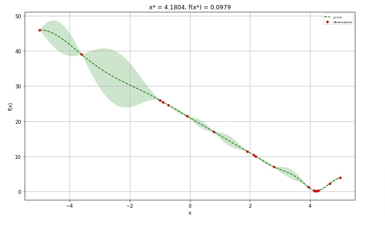
5.1 Gaussian Process and Optimization Results for 1D Objective Functions¶

The first chart that we'll explain plots the whole gaussian optimization process. It'll show a list of values tried as the x-axis and the result of the objective function as the y-axis.

NOTE: This plot will only work for objective functions which accept only one hyperparameter to optimize.

We can create this plot using plot_gaussian_process() method of plots module. It accepts result object (scipy.optimize.OptimizeResult) and created plot from it.

In our case, only our first line formula had one hyperparameter to optimize hence we'll be able to plot only results from it.

Below we have plotted the chart using res2 object from our first example.

The red dot represents the number of different values of x tried and objective function value for those x values.

The dotted line represents the direction followed by the Gaussian process in trying the different values of x.

We can notice that it tried many different values of x at the bottom where it thought trying different values will minimize objective function furthermore.

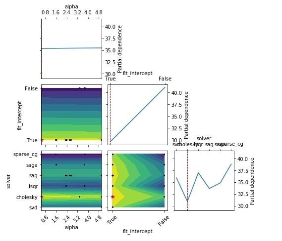
5.2 Partial Dependence Plots of Objective Function¶

The second chart that we'll introduce is a 2D matrix of partial dependence plots of the objective function. It can be used to analyze how each individual hyperparameter is affecting objective function.

We can create this plot using plot_objective() method from plots module. The function takes as input result object (scipy.optimize.OptimizeResult) and creates a plot based on it. The chart on diagonal shows impact of single hyperparameter on objective function whereas all other chart shows the effect of two hyperparameters on the objective function.

Below we have created a plot using the result object from the regression problem section. The chart on diagonal shows the impact of hyperparameters alpha, fit_intercept and solver on the objective function. The charts, other than diagonal show the impact of two hyperparameters combinations.

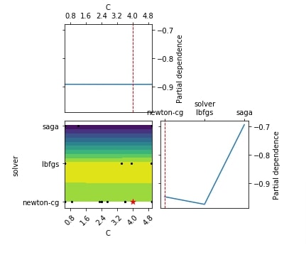
Below we have created another plot partial dependence charts of the objective function with only two hyperparameters (C and solver) using the result object from the classification problem section.

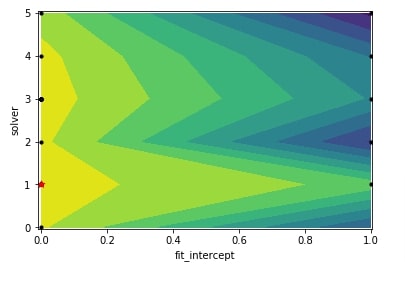
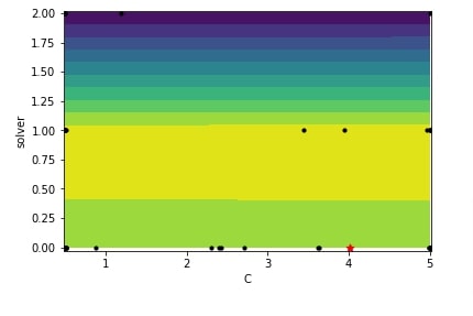
5.3 Partial Dependence Plot of 2 Hyperparameters Combination¶

The plots module provide a separate method name plot_objective_2D() if we want to create a partial dependence plot of objective function based on two hyperparameters. We need to provide a method with the result object (scipy.optimize.OptimizeResult) and the name of two hyperparameters based on which we want to create a partial dependence plot.

Below we have created a partial dependence plot showing the effect of hyperparameters fit_intercept and solver on an objective function from the regression problem section.

Below we have created another partial dependence plot showing the effect of hyperparameters C and solver on objective function from the classification problem section.

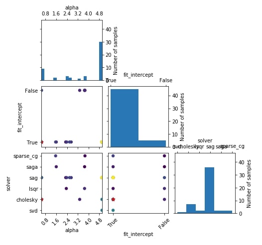
5.4 Hyperparameters Search Space Sampling Plot¶

In this section, we'll introduce a plot that shows how values of hyperparameters were sampled from a list of values or ranges.

The plot is a 2D matrix where charts on diagonal are histograms showing the distribution of values sampled for a particular hyperparameter whereas other charts are scatter plots showing values sampled for combinations of two hyperparameters.

We can create this plot using plot_evaluations() method of plots module by giving result object (scipy.optimize.OptimizeResult) to it. If we want to create plot of only few selected hyperparameters then we can give list of hyperparameter names to plot_dims parameter of the plot_evaluations() method.

Below we have created hyperparameters search space sampling plot for the regression problem section.

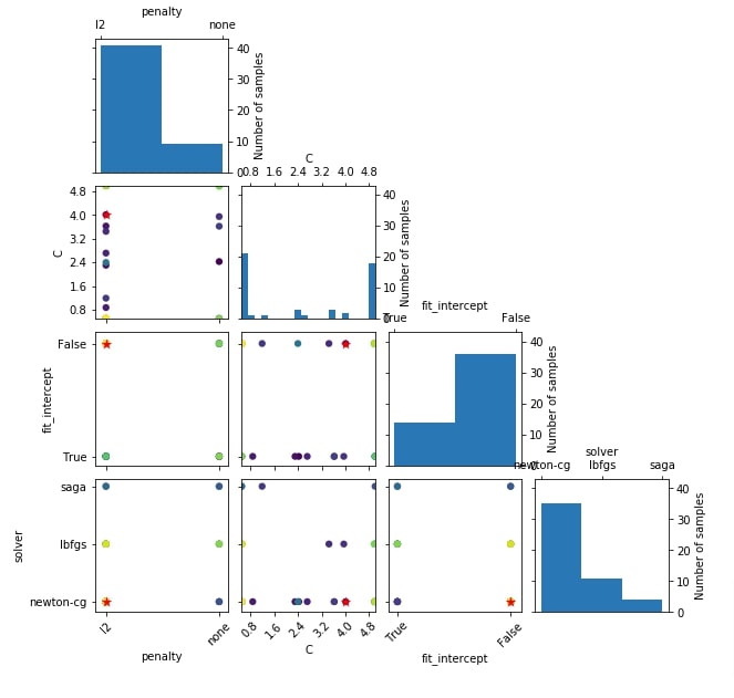
Below we have created another hyperparameter search space sampling plot using the result object from the classification problem section.

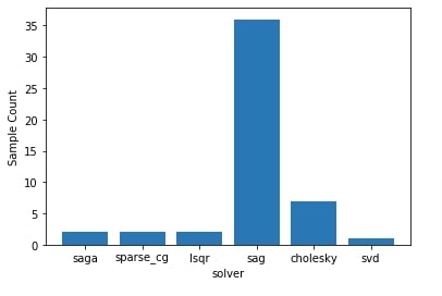
5.5 Hyperparameter Search Space Sampling Histogram¶

We can create a histogram of values sampled for a single hyperparameter only as well.

This is the histogram that gets included on diagonal in the plot created using plot_evaluations() (previous chart).

We can create a histogram of a single hyperparameter's sampled values using plot_histogram() method. We need to provide the result object (scipy.optimize.OptimizeResult) and the hyperparameter name to it.

Below we have created a histogram showing how values of hyperparameters solver were sampled during the optimization process performed in the regression problem section.

We can notice that solver named sag seems to have been sampled more than others as it might be giving good results.

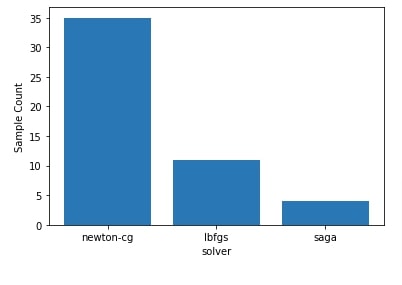
Below we have created another histogram showing distribution of values sampled for hyperparameter solver during the optimization process of the classification problem section.

We can notice that it has sampled solver named newton-cg more compared to others as it might be giving good results.

5.6 Convergence Plot¶

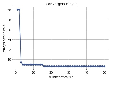
The convergence plot shows how we converged to the minimum value of an objective function over the number of different trials of hyperparameter combinations. The x-axis shows the number of calls to the objective function and the y-axis shows the minimum value of the objective function after that many calls.

We can create convergence plot using plot_convergence() method of plots module by giving result object (scipy.optimize.OptimizeResult) to it.

Below we have created a convergence plot using the result object from the regression problem section. We can notice that it seems to have converged after 15-17 trials and after that metric value returned from the objective function is not decreasing any more.

We can come to the conclusion that trials performed after the first 15-17 trials were not able to reduce the value of the optimization function. We can avoid extra calls to the objective function if the metric value is not decreasing after a particular number of calls which can save time and resources.

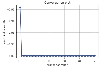
Below we have created a convergence plot using the result object from the classification problem section. We can notice that it seems to have achieved 100% accuracy after first around 5 trials only.

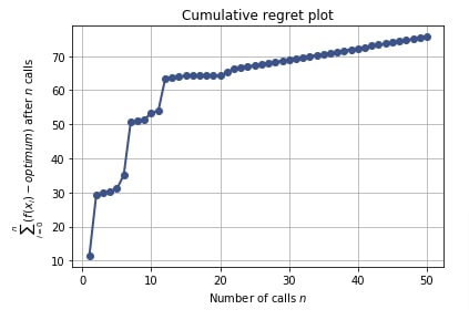
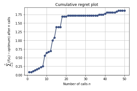
5.7 Cumulative Regret Plot¶

Regret plot shows regret of not sampling best hyperparameters settings.

Regret refers to mistakes in sampling particular hyperparameters combinations which has given bad results. It can help make better decisions on sampling for upcoming trials.

The regret in regret plot is different between total loss accumulated till now minus the minimum loss of all trials till now.

If the line represented by the cumulative plot flattens over time then we can be sure that we are making less or no mistake in sampling hyperparameters.

We can create regret plot using plot_regret() method by giving result object (scipy.optimize.OptimizeResult) to it.

Below we have created a cumulative regret plot using the result object from the regression problem section.

Below we have created another cumulative regret plot using the result object from the classification problem section.

This ends our small tutorial explaining the usage of scikit-optimize library.

References ¶

Other Python Libraries for Hyperparameters Tuning¶

• Optuna
• Hyperopt
• bayes_opt
• Keras-Tuner
• Scikit-learn: Grid Search