Scikit-Learn - Cross-Validation & Hyperparameter Tuning Using Grid Search & Randomized Search
Table of Contents
1. Cross Validation 
We generally split our dataset into train and test sets. We then train our model with train data and evaluate it on test data. This kind of approach lets our model only see a training dataset which is generally around 4/5 of the data.
A better way to generalize the performance of the model is cross-validation as it lets us use more data. In cross-validation, various models are built using different training and non-overlapping test sets. Performance on test sets is then aggregated for better results.
Image Explaining 5-Fold Cross Validation

import numpy as np
import pandas as pd
import matplotlib.pyplot as plt

import sklearn

from collections import Counter

np.set_printoptions(precision=2)

%matplotlib inline
Default Classification Tasks Approach 
Below we are trying the default approach to classification tasks where we divide data into train/test sets, train model, and evaluate it on the test set. We are trying only one combination of the dataset without any kind of cross-validation. It does not explore data fully hence can result in the less generic model.
from sklearn import datasets

iris = datasets.load_iris()
X_iris, Y_iris = iris.data, iris.target
print('Dataset Size : ', X_iris.shape, Y_iris.shape)
Splitting Datasets Into Train/Test Sets
from sklearn.model_selection import train_test_split

X_train, X_test, Y_train, Y_test = train_test_split(X_iris, Y_iris, train_size=0.80, test_size=0.20, random_state=12, stratify=Y_iris)
print('Train/Test Sizes : ',X_train.shape, X_test.shape, Y_train.shape, Y_test.shape)
Training Model
from sklearn.neighbors import KNeighborsClassifier

knn = KNeighborsClassifier()
knn.fit(X_train, Y_train)
Evaluating Model On Test Set.
print('Train Accuracy : %.2f'%knn.score(X_train, Y_train))
print('Test Accuracy : %.2f'%knn.score(X_test, Y_test))
Default Regression Tasks Approach 
Below we are trying the default approach to regression tasks where we divide data into train/test sets, train model, and evaluate it on the test set. We are trying only one combination of the dataset without any kind of cross-validation. It does not explore data fully hence can result in the less generic model.
boston = datasets.load_boston()
X_boston, Y_boston = boston.data, boston.target
print('Dataset Size : ', X_boston.shape, Y_boston.shape)
Splitting Datasets Into Train/Test Sets
from sklearn.neighbors import KNeighborsRegressor

X_train, X_test, Y_train, Y_test = train_test_split(X_boston, Y_boston, train_size=0.80, test_size=0.20, random_state=12)
print('Train/Test Sizes : ',X_train.shape, X_test.shape, Y_train.shape, Y_test.shape)
Training Model
knn = KNeighborsRegressor()
knn.fit(X_train, Y_train)
Evaluating Model On Test Set.
print('Train R^2 Score : %.2f'%knn.score(X_train, Y_train))
print('Test R^2 Score : %.2f'%knn.score(X_test, Y_test))
The above implementation considers only one set of train and test sets. It has not seen the whole dataset. We might get even better results if we try a few other possible combinations of train/test splits. Hence it’s worth trying various combinations to find out good results that generalize well.
sklearn also provides various splitting strategies as mentioned below:
- KFold
- StratifiedKFold
- ShuffleSplit
- StratifiedShuffleSPlit
sklearn provides cross_val_score method which tries various combinations of train/test splits and produces results of each split test score as output.
sklearn also provides a cross_validate method which is exactly the same as cross_val_score except that it returns a dictionary which has fit time, score time and test scores for each splits.
We are trying below StratifiedKFold and StratifiedShuffleSplit for classification dataset(iris) and KFold and ShuffleSplit for regression dataset(boston).
KFold 
K-Fold cross-validation is quite common cross-validation. In K-Fold CV, the total dataset is generally divided into 5/10 folds and then for each iteration of model training, one fold is taken as the test set and remaining folds are combined to the created train set.
from sklearn.model_selection import cross_val_score, cross_validate
from sklearn.model_selection import KFold,StratifiedKFold, ShuffleSplit, StratifiedShuffleSplit
print('Classifying Without Any Cross Validation : ', cross_val_score(KNeighborsRegressor(), X_boston, Y_boston, cv=5)) # Default KFold CV
print('Classifying With KFold Cross Validation : ', cross_val_score(KNeighborsRegressor(), X_boston, Y_boston, cv=KFold(n_splits=5)))
print('Classifying Without Any Cross Validation : \n', cross_validate(KNeighborsRegressor(), X_boston, Y_boston, cv=5)) # Default KFold CV
print('\nClassifying With KFold Cross Validation : \n', cross_validate(KNeighborsRegressor(), X_boston, Y_boston, cv=KFold(n_splits=5)))
We are trying to split the IRIS classification dataset with KFold. Notice that we are also printing each class distribution in train and test sets after splits. Please make a note that class distribution is not proper in training and test sets. By class distribution, we mean that each class of classification dataset has the same amount of presence in both train and test sets. It means that if one class is representing 30% samples of the whole dataset then in both train and test sets it should have 30% representation.
Hence we should generally use StratifiedKFold for classification datasets and KFold for regression datasets.
kfold = KFold(n_splits=5)
masks = []
for i, (train_indexes, test_indexes) in enumerate(kfold.split(X_iris)):
    mask = np.array([(False if j in train_indexes else True) for j in range(len(Y_iris))])
    print('Split[%d] Train Index Distribution by class : '%(i+1),np.bincount(Y_iris[train_indexes])/len(Y_iris))
    print('Split[%d] Test Index Distribution by class : '%(i+1), np.bincount(Y_iris[test_indexes])/len(Y_iris))
    masks.append(mask)
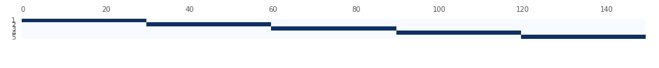
Visualizing Splits Of KFold
Below we are visualizing splits created by KFold from the previous step. We had maintained how it split data at each step into train and test data. Please make a note from the plot that Y-axis represents a split number. We can notice that in the first split it took the first 30 samples as the test set and remaining 120 samples as a train set. We then select the next 30 samples as the train set in the next iteration and so on.
with plt.style.context(('seaborn', 'ggplot')):
    plt.matshow(masks, cmap=plt.cm.Blues, fignum=1)
    plt.yticks(range(5), range(1,6))
    plt.grid(None);
StratifiedKFold 
The StratifiedKFold is commonly used for classification tasks. It works almost like KFold with the only difference that it maintains class distribution the same in train/test sets as that of original dataset distribution. So if we have one class which has a 30% sample in the original dataset then when we split it into train/test sets, both train and test sets will also have a 30% distribution of this class.
print('Classifying Without Any Cross Validation : ', cross_val_score(KNeighborsClassifier(), X_iris, Y_iris, cv=5)) ## It uses StratifiedKFold default
print('Classifying With Stratified KFold Cross Validation : ', cross_val_score(KNeighborsClassifier(), X_iris, Y_iris, cv=StratifiedKFold(n_splits=5)))
print('Classifying Without Any Cross Validation : \n', cross_validate(KNeighborsClassifier(), X_iris, Y_iris, cv=5)) ## It uses StratifiedKFold default
print('\nClassifying With Stratified KFold Cross Validation : \n', cross_validate(KNeighborsClassifier(), X_iris, Y_iris, cv=StratifiedKFold(n_splits=5)))
cross_val_score method will first divide the dataset into the first 5 folds and for each iteration, it takes one of the fold as the test set and other folds as a train set. It generally uses KFold by default for creating folds for regression problems and StratifiedKFold for classification problems.
We are trying to split the classification dataset with StratifiedKFold. Notice that we are also printing each class distribution in train and test sets after splits. Here we can note that class distribution is proper in train and test sets.
skfold = StratifiedKFold(n_splits=5)
masks = []
for i, (train_indexes, test_indexes) in enumerate(skfold.split(X_iris, Y_iris)):
    print('Split[%d] Train Index Distribution by class : '%(i+1),np.bincount(Y_iris[train_indexes])/len(Y_iris))
    print('Split[%d] Test Index Distribution by class : '%(i+1), np.bincount(Y_iris[test_indexes])/len(Y_iris))
    mask = np.array([(False if j in train_indexes else True) for j in range(len(Y_iris))])
    masks.append(mask)
Visualizing Splits Of StratifiedKFold
Below we are visualizing splits created by StratifiedKFold from the previous step. We had maintained how it split data at each step into train and test data. Please make a note from the plot that Y-axis represents a split number. We can notice that in the first split it took the first 30 samples as the test set and remaining 120 samples as train set while maintaining class proportion as well. We then select the next 30 samples as the train set in the next iteration and so on.
with plt.style.context(('seaborn', 'ggplot')):
    plt.matshow(masks, cmap=plt.cm.Blues)
    plt.yticks(range(5), range(1,6))
    plt.grid(None);

ShuffleSplit 
The ShuffleSplit as its name suggests splits dataset based on randomly selected indices. It's commonly used for regression tasks.
print('Classifying Without Any Cross Validation : ', cross_val_score(KNeighborsRegressor(), X_boston, Y_boston, cv=5)) # Default KFold CV
print('Classifying With ShuffleSplit Cross Validation : ', cross_val_score(KNeighborsRegressor(), X_boston, Y_boston, cv=ShuffleSplit(n_splits=5)))
print('Classifying Without Any Cross Validation : \n', cross_validate(KNeighborsRegressor(), X_boston, Y_boston, cv=5)) # Default KFold CV
print('\nClassifying With ShuffleSplit Cross Validation : \n', cross_validate(KNeighborsRegressor(), X_boston, Y_boston, cv=ShuffleSplit(n_splits=5)))
We are trying to split the classification dataset with ShuffleSplit. Notice that we are also printing each class distribution in train and test sets after splits. Please make a note that class distribution is not proper in training and test sets. Hence we should generally use StratifiedShuffleSplit for classification datasets and ShuffleSplit for regression datasets.
shuffle_split = ShuffleSplit(n_splits=5)
masks = []
for i, (train_indexes, test_indexes) in enumerate(shuffle_split.split(X_iris)):
    print('Split[%d] Train Index Distribution by class : '%(i+1),np.bincount(Y_iris[train_indexes])/len(Y_iris))
    print('Split[%d] Test Index Distribution by class : '%(i+1), np.bincount(Y_iris[test_indexes])/len(Y_iris))
    mask = np.array([(False if j in train_indexes else True) for j in range(len(Y_iris))])
    masks.append(mask)
Visualizing Splits Of ShuffleSplit
We can notice from below visualization that ShuffleSplit selected samples randomly unlike KFold which selects samples serially.
with plt.style.context(('seaborn', 'ggplot')):
    plt.matshow(masks, cmap=plt.cm.Blues)
    plt.yticks(range(5), range(1,6))
    plt.grid(None);

StratifiedShuffleSplit 
The StratifiedShuffleSplit works exactly like ShuffleSplit but designed for classification tasks where we need to maintain class proportion after splitting of data.
print('Classifying Without Any Cross Validation : ', cross_val_score(KNeighborsClassifier(), X_iris, Y_iris, cv=5)) ## It uses StratifiedKFold default
print('Classifying With StratifiedShuffleSplit Cross Validation : ', cross_val_score(KNeighborsClassifier(), X_iris, Y_iris, cv=StratifiedShuffleSplit(n_splits=5)))
print('Classifying Without Any Cross Validation : \n', cross_validate(KNeighborsClassifier(), X_iris, Y_iris, cv=5)) ## It uses StratifiedKFold default
print('\nClassifying With StratifiedShuffleSplit Cross Validation : \n', cross_validate(KNeighborsClassifier(), X_iris, Y_iris, cv=StratifiedShuffleSplit(n_splits=5)))
We are trying to split the classification dataset with StratifiedShuffleSplit. Notice that we are also printing each class distribution in train and test sets after splits. Here we can note that class distribution is proper in train and test sets.
shuffle_split = StratifiedShuffleSplit(n_splits=5)
masks = []
for i, (train_indexes, test_indexes) in enumerate(shuffle_split.split(X_iris, Y_iris)):
    print('Split[%d] Train Index Distribution by class : '%(i+1),np.bincount(Y_iris[train_indexes])/len(Y_iris))
    print('Split[%d] Test Index Distribution by class : '%(i+1), np.bincount(Y_iris[test_indexes])/len(Y_iris))
    mask = np.array([(False if j in train_indexes else True) for j in range(len(Y_iris))])
    masks.append(mask)
Visualising Splits Of StratifiedShuffleSplit
with plt.style.context(('seaborn', 'ggplot')):
    plt.matshow(masks, cmap=plt.cm.Blues)
    plt.yticks(range(5), range(1,6))
    plt.grid(None);

sklearn also provides validatation_curve method which can take single hyperparameters and list of various values for that hyperparameters, then it returns train and test scores for various cross-validation folds. It's generally used for plotting purposes.
from sklearn.model_selection import validation_curve

n_neighbors = [1, 3, 5, 10, 20, 50]
train_scores, test_scores = validation_curve(KNeighborsRegressor(), X_iris, Y_iris, param_name="n_neighbors",
                                             param_range=n_neighbors, cv=StratifiedShuffleSplit(n_splits=5, random_state=123))

with plt.style.context(('seaborn', 'ggplot')):
    plt.plot(n_neighbors, train_scores.mean(axis=1), label="train accuracy")
    plt.plot(n_neighbors, test_scores.mean(axis=1), label="test accuracy")
    plt.ylabel('Accuracy')
    plt.xlabel('Number of neighbors')
    #plt.xlim([50, 0])
    plt.legend(loc="best");

2. Hyperparameter Tuning Using Grid Search & Randomized Search 
All complex machine learning model has more than one hyperparameters. Most of the models have default values set for these parameters. If we fit train data with the default model then it might happen that it does not fit data well. It can overfit data or underfit data as well. We need to find a proper trade-off between overfitting & underfit by doing grid search through various values of hyperparameters of the model.
Grid Search does try the list of all combinations of values given for a list of hyperparameters with model and records the performance of model based on evaluation metrics and keeps track of the best model and hyperparameters as well. We can try all parameters by writing a loop inside a loop for each hyperparameter values.
X_train, X_test, Y_train, Y_test = train_test_split(X_boston, Y_boston,
                                                    train_size=0.80,
                                                    test_size=0.20,
                                                    random_state=12)
from sklearn.ensemble import RandomForestRegressor

best_score = 0.0
best_params = {'max_depth': None, 'max_features': 'auto','n_estimators': 10}
for max_depth in [None, 2,3,5]:
    for max_features in ['auto','sqrt', 'log2']:
        for n_estimators in [10,100]:
            score = cross_val_score(RandomForestRegressor(n_estimators=n_estimators,
                                                          max_features=max_features,
                                                          max_depth=max_depth,
                                                          random_state=123
                                                          ),
                                    X_train,
                                    Y_train,
                                    cv=ShuffleSplit(n_splits=5, random_state=123),
                                    n_jobs=-1).mean()
            if score > best_score:
                best_score= score
                best_params['max_depth'],best_params['max_features'], best_params['n_estimators'] = max_depth, max_features, n_estimators

            print('max_depth : %s, max_features : %s, n_estimators : %s , Average R^2 Score : %.2f'%(str(max_depth), max_features, str(n_estimators), score))

print('\nBest Score : %.2f, Best Params : %s'%(best_score, str(best_params)))
rf_best = RandomForestRegressor(**best_params)
rf_best.fit(X_train, Y_train)

print("Test R^2 Score : ", rf_best.score(X_test, Y_test))
GridSearchCV 
sklearn provides GridSearchCV class which takes a list of hyperparameters and their values as a dictionary and will try all combinations on the model and also will keep track of results as well for each Cross-Validation Folds.
from sklearn.model_selection import GridSearchCV, RandomizedSearchCV

grid = GridSearchCV(RandomForestRegressor(random_state=123),
                    param_grid = {'max_depth': [None, 2,3,5], 'max_features' : ['auto','sqrt', 'log2'], 'n_estimators': [10,100],},
                    cv = ShuffleSplit(n_splits=5, random_state=123),
                    verbose=50,
                    n_jobs=-1)

grid.fit(X_train, Y_train)

print('\nBest R^2 Score : %.2f'%grid.best_score_, ' Best Params : ', str(grid.best_params_))
Grid objects also keep tracks of all hyperparameters tried on all cross-validation splits along with information about their score, fit times, mean scores, standard scores, mean fit times, standard fit times. It also ranks models best on performance with best models ranked 1 and next one 2 and so on.
grid.cv_results_.keys()
pd.DataFrame(grid.cv_results_)[['param_max_depth', 'param_max_features', 'param_n_estimators','mean_test_score', 'rank_test_score']]
Grid object also keeps the best model available as the best_estimator_ parameter so that it can be used for prediction purposes further.
grid.best_estimator_
print('First Few preds : ', grid.predict(X_boston)[:5])
print('Actual Values   : ', Y_boston[:5])
print("Test R^2 Score : ", grid.score(X_test, Y_test))
RandomizedSearchCV 
The RandomizedSearchCV is another approach of performing hyperparameter tunning. Unlike GridSearchCV which tries all possible parameter settings passed to it, RandomizedSearchCV tries only a specified number of parameter settings from total parameter search space. It accepts a parameter named n_iter (integer) which lets RandomizedSearchCV select that many parameter settings from all possible parameter settings to try on model. Below we are explaining the usage of it using Boston housing dataset that was split into train/test sets when explaining GridSearchCV.
from sklearn.model_selection import RandomizedSearchCV

grid = RandomizedSearchCV(RandomForestRegressor(random_state=123), n_iter=5,
                    param_distributions = {'max_depth': [None, 2,3,5], 'max_features' : ['auto','sqrt', 'log2'], 'n_estimators': [10,100],},
                    cv = ShuffleSplit(n_splits=5, random_state=123),
                    verbose=50,
                    n_jobs=-1)

grid.fit(X_train, Y_train)

print('\nBest R^2 Score : %.2f'%grid.best_score_, ' Best Params : ', str(grid.best_params_))
We can notice from the above output that even though a possible number of parameter settings is quite high but it only tries 5 different parameter settings. It’s showing total 25 fits because it'll do cross-validation with 5 splits per each parameter setting.
Below we are printing results of each parameter setting converted to pandas dataframe.
pd.DataFrame(grid.cv_results_)[['param_max_depth', 'param_max_features', 'param_n_estimators','mean_test_score', 'rank_test_score']]
grid.best_estimator_
print('First Few preds : ', grid.predict(X_boston)[:5])
print('Actual Values   : ', Y_boston[:5])
print("Test R^2 Score : ", grid.score(X_test, Y_test))
This ends our small tutorial on cross-validation and hyperparameter tunning using a grid search using scikit-learn. Please feel free to let us know your views in the comments section.
References 
 Sunny Solanki
Sunny Solanki
Intro: Software Developer | Youtuber | Bonsai Enthusiast
About: Sunny Solanki holds a bachelor's degree in Information Technology (2006-2010) from L.D. College of Engineering. Post completion of his graduation, he has 8.5+ years of experience (2011-2019) in the IT Industry (TCS). His IT experience involves working on Python & Java Projects with US/Canada banking clients. Since 2020, he’s primarily concentrating on growing CoderzColumn.
His main areas of interest are AI, Machine Learning, Data Visualization, and Concurrent Programming. He has good hands-on with Python and its ecosystem libraries.
Apart from his tech life, he prefers reading biographies and autobiographies. And yes, he spends his leisure time taking care of his plants and a few pre-Bonsai trees.
Contact: sunny.2309@yahoo.in


![YouTube Subscribe]() Comfortable Learning through Video Tutorials?
Comfortable Learning through Video Tutorials?
If you are more comfortable learning through video tutorials then we would recommend that you subscribe to our YouTube channel.
![Need Help]() Stuck Somewhere? Need Help with Coding? Have Doubts About the Topic/Code?
Stuck Somewhere? Need Help with Coding? Have Doubts About the Topic/Code?
 Stuck Somewhere? Need Help with Coding? Have Doubts About the Topic/Code?
When going through coding examples, it's quite common to have doubts and errors.
If you have doubts about some code examples or are stuck somewhere when trying our code, send us an email at coderzcolumn07@gmail.com. We'll help you or point you in the direction where you can find a solution to your problem.
You can even send us a mail if you are trying something new and need guidance regarding coding. We'll try to respond as soon as possible.
![Share Views]() Want to Share Your Views? Have Any Suggestions?
Want to Share Your Views? Have Any Suggestions?
 Want to Share Your Views? Have Any Suggestions?
If you want to
- provide some suggestions on topic
- share your views
- include some details in tutorial
- suggest some new topics on which we should create tutorials/blogs
 sklearn, cross-validation, grid-search