Updated On : Apr-19,2020 Time Investment : ~30 mins

Styling, Theming and Annotation of Bokeh Plots [Python]¶

Table of Contents¶

Introduction
Loading Dataset
1. Colors
2. Graph Properties
3. Plot Properties
4. Grids Configuration Attributes
5. Legends Configuration Attributes
6. Toolbar Configuration Attributes
7. Box Annotations Configuration
8. Labels Annotations Configuration
References

Introduction ¶

Our first tutorial on bokeh concentrated on basic plotting with bokeh but lacked information about various styling functionalities available in bokeh. If you want to learn about basic glyphs plotting with bokeh then we suggest that you go through that tutorial. Bokeh provides a rich set of attributes and methods which can be used to improve the visual appearance of data visualization. We'll be discussing styling, theming and annotation functionalities available in bokeh as a part of this tutorial.

So without further delay, let’s start with the tutorial.

We'll start by importing our default imports.

from bokeh.io import output_notebook, show
from bokeh.plotting import figure
from bokeh.resources import INLINE

output_notebook(resources=INLINE)

Loading Dataset ¶

We need to load datasets which we'll be using for our purpose through this tutorial. Bokeh provides a list of datasets as pandas dataframe as a part of it's bokeh.sampledata module. The first dataset that, we'll be using is autompg dataset which has information about car models along with their mpg, no of cylinders, disposition, horsepower, weight. acceleration, year launched, origin, name, and manufacturer.

from bokeh.sampledata.autompg import autompg_clean as autompg_df
autompg_df.head()

	mpg	cyl	displ	hp	weight	accel	yr	origin	name	mfr
0	18.0	8	307.0	130	3504	12.0	70	North America	chevrolet chevelle malibu	chevrolet
1	15.0	8	350.0	165	3693	11.5	70	North America	buick skylark 320	buick
2	18.0	8	318.0	150	3436	11.0	70	North America	plymouth satellite	plymouth
3	16.0	8	304.0	150	3433	12.0	70	North America	amc rebel sst	amc
4	17.0	8	302.0	140	3449	10.5	70	North America	ford torino	ford

Another dataset that we'll be using for our purpose is google stock dataset which has information about stock open, high, low, close prices per business day as well as daily volume data.

from bokeh.sampledata.stocks import GOOG as google
import pandas as pd

google_df = pd.DataFrame(google)
google_df["date"] = pd.to_datetime(google_df["date"])
google_df.head()

	date	open	high	low	close	volume	adj_close
0	2004-08-19	100.00	104.06	95.96	100.34	22351900	100.34
1	2004-08-20	101.01	109.08	100.50	108.31	11428600	108.31
2	2004-08-23	110.75	113.48	109.05	109.40	9137200	109.40
3	2004-08-24	111.24	111.60	103.57	104.87	7631300	104.87
4	2004-08-25	104.96	108.00	103.88	106.00	4598900	106.00

1. Colors ¶

Bokeh lets us provide color details at various places when constructing graphs. It lets us provide color details in different ways as mentioned below.

named colors
an RGB(A) hex value (#FF0000, #44444444, etc)
(r,g,b) tuple (values between 0-255)
(r,g,b,a) tuple (r,g and b values between 0-255 and a between 0-1) We can pass these color values to various graph properties which we'll discuss next.

2. Graph Properties ¶

Bokeh provides three kinds of properties that can be used to modify various aspects of the graph.

Line Properties - Lets us modify the appearance of lines.
- line_color - Line color
- line_width - Line width in pixels
- line_alpha - Line transparency between 0-1 (floating point)
- line_dash - Type of Line. (solid, dashed, dotted, dashdot, etc)
Fill Properties - Lets us modify appearance of filled area.
- fill_color - Color of glyph areas like circle, rectangle, etc
- fill_alpha - Color transparency of glyph areas like circle, rectangle, etc
Text Properties - Lets us modify the appearance of the text of graph.
- text_font - Font family (times, helvetica, etc)
- text_font_size - Font size in pixels, em. (2px, 2em, etc)
- text_font_style - Font style (normal, italic and bold)
- text_color - Color of text
- text_alpha - Transparency of text color (float between 0-1)
- text_align - Text Alignment (left, right, center)
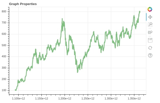
We'll not try the above-mentioned attributes on various plots through examples. Below we are plotting the line chart of google stock prices over time.

fig = figure(width=600, height=400, title="Graph Properties")

fig.line(x=google_df.date, y=google_df.close,
         line_color="green",
         line_width=3,
         line_alpha=0.5,
         #line_dash="dashed",
         )

show(fig)

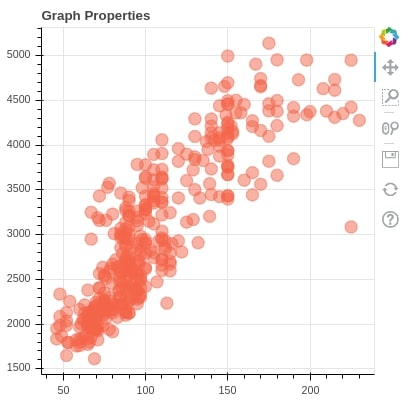
Below we are plotting another scatter plot showing the relation between horsepower and weight of cars in autompg dataset. We are also modifying various graph properties as well to change graph styling.

fig = figure(width=400, height=400, title="Graph Properties")

fig.circle(x=autompg_df.hp, y=autompg_df.weight,
           size=12,
           fill_color="tomato",
           fill_alpha=0.5,
           line_color="tomato",
           line_alpha=0.5,
          )

show(fig)

3. Plot Properties ¶

Many plot level properties like title text, color, axes color, plot lines, etc can be modified as well according to our needs. We'll explain a few graph properties modification with example. The majority of properties of the plot has the same name as the above properties.

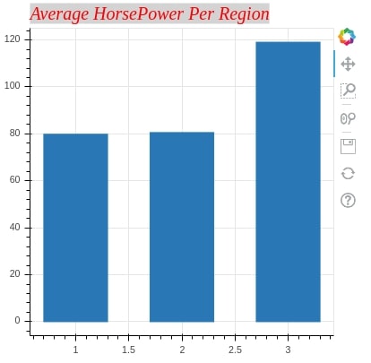
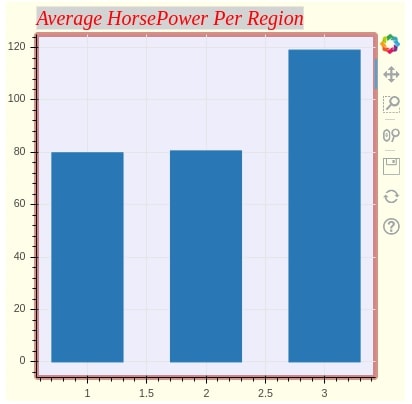
3.1 Title Configuration Attributes ¶

Below we are explaining various attributes to change plot title configuration. We can access the title object from the figure object and then modify its attributes.

avg_autompg = autompg_df.groupby(by="origin").mean().reset_index()

fig = figure(width=400, height=400)

bar = fig.vbar(x=[1,2,3], width=0.6, top=avg_autompg.hp)

fig.title.text="Average HorsePower Per Region"
fig.title.text_font = "times new roman"
fig.title.text_color="red"
fig.title.text_font_style="italic"
fig.title.text_font_size="20px"
fig.title.background_fill_color="lightgrey"



show(fig)

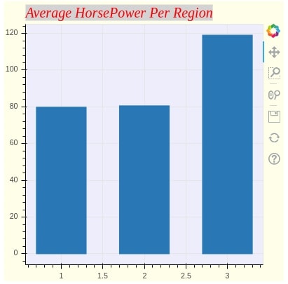
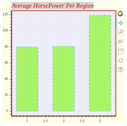
3.2 Background Configuration Attributes ¶

Below we are adding a few further configurations to change plot background configuration. We can set various background attributes by accessing them through the figure object.

fig.background_fill_color="lavender"
fig.background_fill_alpha=0.7
fig.border_fill_color="lightyellow"
fig.border_fill_alpha=0.7

show(fig)

3.3 Plot Outline and Border Configuration Attributes ¶

Below we are further adding few more attributes for configuration of plot borders. We can modify border attributes by accessing them through figure object as well.

fig.min_border_left = 30

fig.outline_line_width = 5
fig.outline_line_alpha = 0.5
fig.outline_line_color = "firebrick"


show(fig)

3.4 Glyph Configuration Attributes ¶

We can modify various graph attributes by accessing the glyph object from graph object and then modifying them.

bar.glyph.fill_color="lawngreen"
bar.glyph.fill_alpha=0.6
bar.glyph.line_width=3
bar.glyph.line_color="skyblue"
bar.glyph.line_alpha=0.8
bar.glyph.line_dash="dashed"


show(fig)

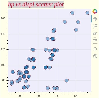
3.5 Axes Configuration Attributes ¶

Axes can be modified by accessing attributes axes, xaxes and yaxis on figure object. Axes properties can be grouped based on usage into the below categories.

axis - Axes Overall Properties (axis_line_width)
axis_label Axes label configuration properties ( axis_label_text_color, axis_label_text_font_size, etc)
major_label Axes major label configuration properties. (major_label_text_font_size, major_label_orientation, etc)
major_tick Axes major tick configuration properties. (major_tick_line_dash, major_tick_in, major_tick_out, etc)
minor_tick Axes minor tick configuration properties. (minor_tick_line_width, minor_tick_in ,minor_tick_out, etc)

We'll try to modify the various axis properties below. We'll also modify graph properties that were introduced earlier. We'll be incrementally adding new properties to the graph.

fig = figure(height=400, width=400, title="hp vs displ scatter plot")

circle = fig.circle(x= autompg_df[autompg_df["origin"]=="Asia"]["hp"],
           y= autompg_df[autompg_df["origin"]=="Asia"]["displ"],
          )

fig.title.text_font = "times new roman"
fig.title.text_color="crimson"
fig.title.text_font_style="italic"
fig.title.text_font_size="25px"
fig.title.background_fill_color="lightgrey"

fig.background_fill_color="lavender"
fig.background_fill_alpha=0.7
fig.border_fill_color="lightyellow"
fig.border_fill_alpha=0.7

fig.background_fill_color="lavender"
fig.background_fill_alpha=0.7
fig.border_fill_color="lightyellow"
fig.border_fill_alpha=0.7

circle.glyph.size=15
circle.glyph.fill_alpha=0.5
circle.glyph.line_width=2
circle.glyph.line_color="darkred"
circle.glyph.line_alpha=0.9
circle.glyph.line_dash="dotted"


show(fig)

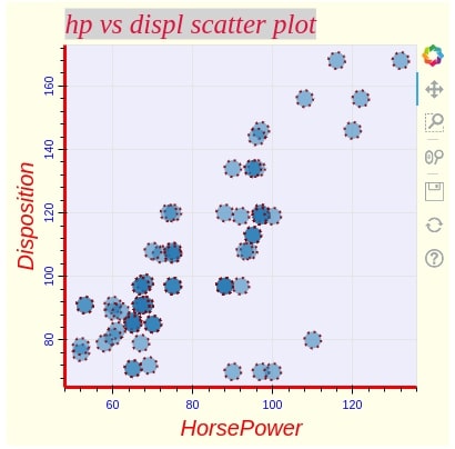
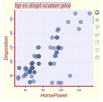
Below we are modifying various x and y-axis attributes to change its styling.

fig.xaxis.axis_label="HorsePower"
fig.xaxis.axis_label_text_color="red"
fig.xaxis.axis_label_text_font_size="20px"
fig.xaxis.major_label_text_color = "blue"
fig.xaxis.axis_line_color="red"
fig.xaxis.axis_line_width=3

fig.yaxis.axis_label="Disposition"
fig.yaxis.axis_label_text_color="red"
fig.yaxis.axis_label_text_font_size="20px"
fig.yaxis.major_label_text_color = "blue"
fig.yaxis.major_label_orientation = "vertical"
fig.yaxis.axis_line_color="red"
fig.yaxis.axis_line_width=3

show(fig)

Below we are modifying major and minor ticker configurations.

fig.xaxis.major_tick_line_color = "blue"
fig.xaxis.major_tick_line_width = 3
fig.xaxis.minor_tick_line_color = "skyblue"
fig.xaxis.minor_tick_line_width = 3

fig.yaxis.major_tick_line_color = "blue"
fig.yaxis.major_tick_line_width = 3
fig.yaxis.minor_tick_line_color = "skyblue"
fig.yaxis.minor_tick_line_width = 3


show(fig)

4. Grids Configuration Attributes ¶

Grids configuration can be modified by accessing attributes grid, xgrid and ygrid on figure object. We'll explain it below with few configuration examples.

fig.xgrid.grid_line_alpha = 0.5
fig.xgrid.grid_line_color = "grey"
fig.ygrid.grid_line_alpha = 0.5
fig.ygrid.grid_line_color = "grey"

show(fig)

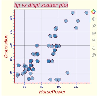
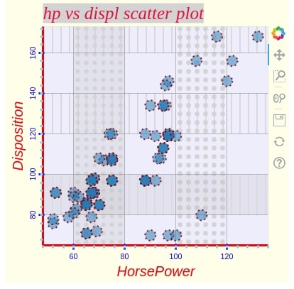
fig.xgrid.band_fill_alpha = 0.1
fig.xgrid.band_fill_color = "grey"
fig.ygrid.band_fill_alpha = 0.1
fig.ygrid.band_fill_color = "grey"

show(fig)

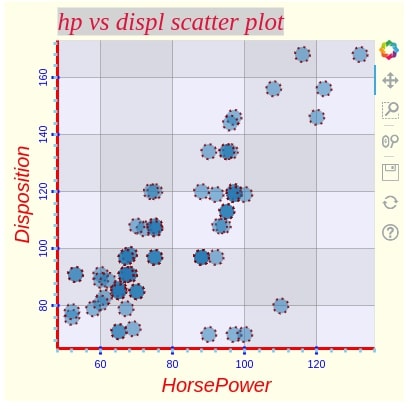
fig.xgrid.band_hatch_pattern = "."
fig.xgrid.band_hatch_color = "lightgrey"
fig.ygrid.band_hatch_pattern = "|"
fig.ygrid.band_hatch_color = "lightgrey"

show(fig)

5. Legends Configuration Attributes ¶

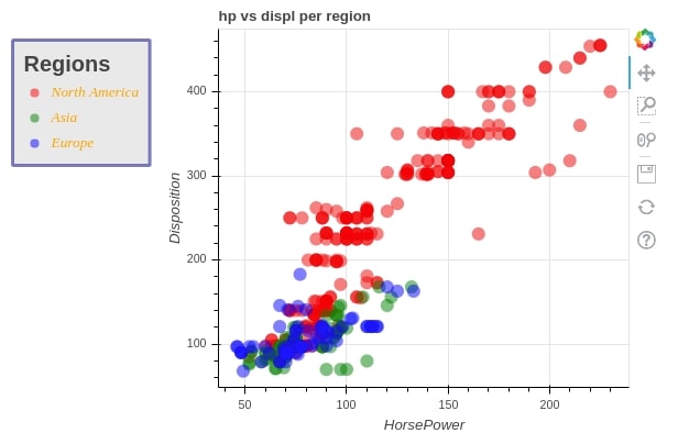
We'll now explain how to modify various configurations of the legends of the graph. We are merging three scatter plots based on three regions of car data available. We can access legend object from the figure object and then modify its attributes.

fig = figure(width=400, height=400, title="hp vs displ per region")

fig.circle(x=autompg_df[autompg_df["origin"]=="North America"]["hp"],
           y=autompg_df[autompg_df["origin"]=="North America"]["displ"],
           fill_color="red", size=12, fill_alpha=0.5, line_width=0,
           legend_label="North America")

fig.circle(x=autompg_df[autompg_df["origin"]=="Asia"]["hp"],
           y=autompg_df[autompg_df["origin"]=="Asia"]["displ"],
           fill_color="green", size=12, fill_alpha=0.5, line_width=0,
           legend_label="Asia")

fig.circle(x=autompg_df[autompg_df["origin"]=="Europe"]["hp"],
           y=autompg_df[autompg_df["origin"]=="Europe"]["displ"],
           fill_color="blue", size=12, fill_alpha=0.5, line_width=0,
           legend_label="Europe")

fig.xaxis.axis_label="HorsePower"
fig.yaxis.axis_label="Disposition"

fig.legend.label_text_font="times"
fig.legend.location = "top_left"
fig.legend.title="Regions"

show(fig)

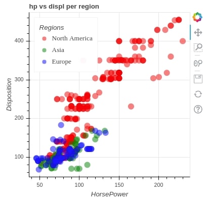
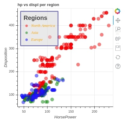
Below we are modifying various text related, border-related and background related properties of legend object.

fig.legend.title_text_font_style = "bold"
fig.legend.title_text_font_size = "15pt"

fig.legend.label_text_font_style = "italic"
fig.legend.label_text_color = "orange"


fig.legend.border_line_width = 3
fig.legend.border_line_color = "navy"
fig.legend.border_line_alpha = 0.5
fig.legend.background_fill_color = "lightgrey"
fig.legend.background_fill_alpha = 0.5

show(fig)

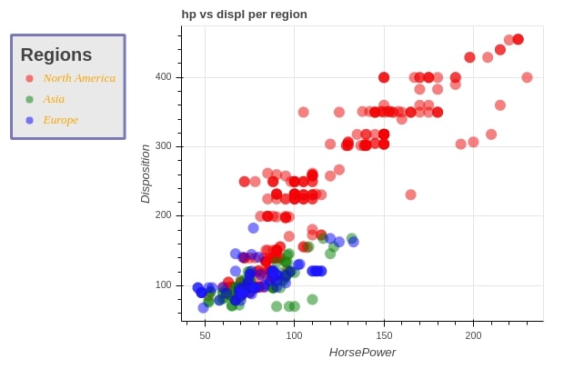
Below we are explaining how to create manual legend instead of using default legend generated by bokeh. We'll be modifying various properties of manual legend as well. We'll be using the Legend class from bokeh.models to create manual legends.

from bokeh.models import Legend

fig = figure(width=600, height=400, title="hp vs displ per region")

c1 = fig.circle(x=autompg_df[autompg_df["origin"]=="North America"]["hp"],
           y=autompg_df[autompg_df["origin"]=="North America"]["displ"],
           fill_color="red", size=12, fill_alpha=0.5, line_width=0)

c2 = fig.circle(x=autompg_df[autompg_df["origin"]=="Asia"]["hp"],
           y=autompg_df[autompg_df["origin"]=="Asia"]["displ"],
           fill_color="green", size=12, fill_alpha=0.5, line_width=0)

c3 = fig.circle(x=autompg_df[autompg_df["origin"]=="Europe"]["hp"],
           y=autompg_df[autompg_df["origin"]=="Europe"]["displ"],
           fill_color="blue", size=12, fill_alpha=0.5, line_width=0)

fig.xaxis.axis_label="HorsePower"
fig.yaxis.axis_label="Disposition"

legend = Legend(items=[
    ("North America"   , [c1]),
    ("Asia" , [c2]),
    ("Europe" , [c3]),
], location="top_left")

fig.add_layout(legend, 'left')

fig.legend.title="Regions"
fig.legend.title_text_font_style = "bold"
fig.legend.title_text_font_size = "15pt"

show(fig)

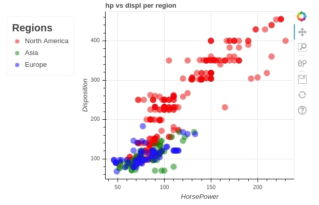
fig.legend.label_text_font = "times"
fig.legend.label_text_font_style = "italic"
fig.legend.label_text_color = "orange"

show(fig)

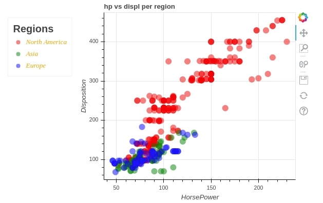
fig.legend.border_line_width = 3
fig.legend.border_line_color = "navy"
fig.legend.border_line_alpha = 0.5
fig.legend.background_fill_color = "lightgrey"
fig.legend.background_fill_alpha = 0.5

show(fig)

We can modify the locations of the toolbar as well as the visibility of the toolbar as well. We are explaining it below with an example.

fig.toolbar_location="above"
fig.toolbar.autohide = True

show(fig)

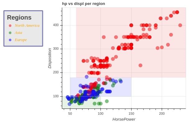
7. Box Annotations Configuration ¶

Below we are explaining how we can use BoxAnnotation to highlight a particular area of the graph. We have highlighted three areas according to three regions which cover most of the points from those regions.

from bokeh.models import BoxAnnotation

low_box = BoxAnnotation(top=100, left=0,right=100, fill_alpha=0.1,  fill_color='green')
mid_box = BoxAnnotation(bottom=100, top=180, left=50,right=150, fill_alpha=0.1, fill_color='blue')
high_box = BoxAnnotation(bottom=180, left=60,fill_alpha=0.1, fill_color='red')

fig.add_layout(low_box)
fig.add_layout(mid_box)
fig.add_layout(high_box)

show(fig)

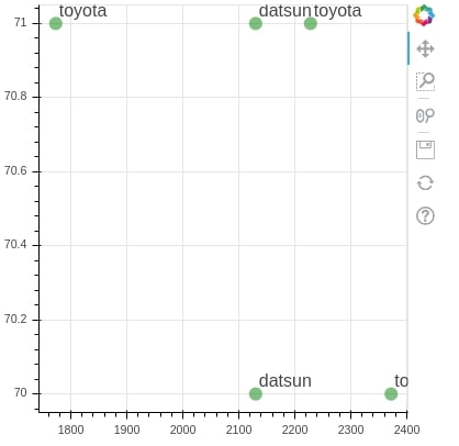
8. Labels Annotations Configuration ¶

We can also label various points in our graph. We are explaining below with example where we are annotating the first 5 cars from Asia region with their names in scatter plot of weight vs manufacturing year.

from bokeh.models import ColumnDataSource, Label, LabelSet

first_5 = autompg_df[autompg_df["origin"]=="Asia"].head(5).drop_duplicates()

fig = figure(width=400, height=400)

c = fig.circle(x=first_5["weight"],
           y=first_5["yr"],
           fill_color="green", size=12, fill_alpha=0.5, line_width=0)

labels = LabelSet(x='weight', y='yr', text='mfr', level='glyph',
              x_offset=3, y_offset=3, source=ColumnDataSource(first_5), render_mode='canvas')

fig.add_layout(labels)

show(fig)

This ends our small tutorial on styling bokeh plots. Please feel free to let us know your views in the comments section.

References ¶

Sunny Solanki

Comfortable Learning through Video Tutorials?

If you are more comfortable learning through video tutorials then we would recommend that you subscribe to our YouTube channel.

Stuck Somewhere? Need Help with Coding? Have Doubts About the Topic/Code?

When going through coding examples, it's quite common to have doubts and errors.

If you have doubts about some code examples or are stuck somewhere when trying our code, send us an email at coderzcolumn07@gmail.com. We'll help you or point you in the direction where you can find a solution to your problem.

You can even send us a mail if you are trying something new and need guidance regarding coding. We'll try to respond as soon as possible.

Want to Share Your Views? Have Any Suggestions?

If you want to

provide some suggestions on topic
share your views
include some details in tutorial
suggest some new topics on which we should create tutorials/blogs

Please feel free to contact us at coderzcolumn07@gmail.com. We appreciate and value your feedbacks. You can also support us with a small contribution by clicking DONATE.

bokeh, stling, theming, annotation

Sunny Solanki

Software Developer | Youtuber | Bonsai Enthusiast

Subscribe to Our YouTube Channel

Tutorial Categories

Artificial Intelligence (83)
Data Science (84)
Digital Marketing (8)
Machine Learning (38)
Python (131)

Styling, Theming and Annotation of Bokeh Plots [Python]¶

Table of Contents¶

Introduction ¶

Loading Dataset ¶

1. Colors ¶

2. Graph Properties ¶

3. Plot Properties ¶

3.1 Title Configuration Attributes ¶

3.2 Background Configuration Attributes ¶

3.3 Plot Outline and Border Configuration Attributes ¶

3.4 Glyph Configuration Attributes ¶

3.5 Axes Configuration Attributes ¶

4. Grids Configuration Attributes ¶

5. Legends Configuration Attributes ¶

6. Toolbar Configuration Attributes ¶

7. Box Annotations Configuration ¶

8. Labels Annotations Configuration ¶

References ¶

Sunny Solanki

Comfortable Learning through Video Tutorials?

Stuck Somewhere? Need Help with Coding? Have Doubts About the Topic/Code?

Want to Share Your Views? Have Any Suggestions?

Sunny Solanki

Subscribe to Our YouTube Channel

Tutorial Categories

Newsletter Subscription