Guide To Use Word Embeddings For Flax (JAX) Text Classification Networks
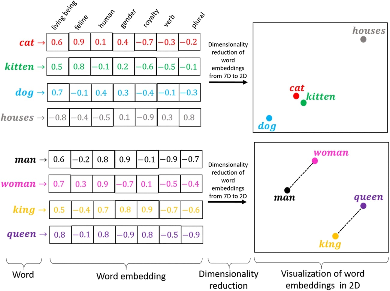
When we want to develop a deep learning or machine learning model that works on text data, we first need to convert text data to floats using some approach as ML/DL models only work with floats. Over the years, many approaches have been developed like word frequency, one-hot encoding of words, TF-IDF (Term Frequency-Inverse Document Frequency), word embeddings, etc. The approaches like word frequency and TF-IDF uses just one float to represent one word/token. This approach works generally well for NLP tasks like text classification involving less data but might not work well with other NLP tasks like text generation that requires understanding the context of the text. As they use just one float per word/token, there is a limitation to the amount of information that can be represented through it. To solve this, word embeddings were invented. In the case of word embeddings, a list of floats (a vector) is used to represent a single word/token which is generally referred to as embeddings of that word/token. This float vector has the capability to capture the meaning of the word better and can also capture contextual information. Generally, when we train and update these embeddings through our networks, embeddings of words that are the same (by meaning or in the same context) will be near to one another.
As a part of this tutorial, we have explained how we can use word embeddings for text classification networks designed using Flax (JAX). The Flax is a high-level Python deep learning library designed on top of JAX to simplify the process of creating neural networks. We have tried various approaches to work with word embeddings. We have used AG NEWS dataset available from torchtext and word tokenizing functionalities available from Keras. Apart from this, we have also explained predictions made by the network using LIME algorithm.
Below, we have listed important sections of tutorial to give an overview of the material covered.
Important Sections Of Tutorial
- Prepare Data
- 1.1 Load Data
- 1.2 Vectorize Data
- Approach 1 - Word Embeddings
- 2.1 Create Network
- 2.2 Define Loss
- 2.3 Train Network
- 2.4 Evaluate Network Performance
- 2.5 Explain Network Predictions Using LIME
- Approach 2 - Word Embeddings With More Values
- Approach 3 - Word Embeddings Averaged
- Approach 4 - Word Embeddings Summed
Below, we have imported the necessary libraries and printed the versions that we have used in our tutorial.
import jax

print("JAX Version : {}".format(jax.__version__))
import flax

print("Flax Version : {}".format(flax.__version__))
import optax

print("OPTAX Version : {}".format(optax.__version__))
import torchtext

print("Torchtext Version : {}".format(torchtext.__version__))
from tensorflow import keras

print("Keras Version : {}".format(keras.__version__))
1. Prepare Data 
In this section, we have prepared data that we'll be feeding to our neural network. We have first loaded the dataset, populated vocabulary (mapping from unique words to indexes) with tokens/words, and then transformed text to a list of token indexes using vocabulary. In the end, we'll have a list of indexes for each text document where indexes are mapped from index to token/word as per our vocabulary. We'll give this list of indexes as input to our network which will then generate embeddings from them and update embeddings as we train it.
1.1 Load Data
Below, we have simply loaded AG NEWS dataset available from PyTorch. The dataset has text documents for 4 different categories of news (["World", "Sports", "Business", "Sci/Tech"]).
| Index | Category |
|---|---|
| 1 | World |
| 2 | Sports |
| 3 | Business |
| 4 | Sci/Tec |
import numpy as np

train_dataset, test_dataset = torchtext.datasets.AG_NEWS()

X_train_text, Y_train = [], []
for Y, X in train_dataset:
    X_train_text.append(X)
    Y_train.append(Y)

X_test_text, Y_test = [], []
for Y, X in test_dataset:
    X_test_text.append(X)
    Y_test.append(Y)

unique_classes = list(set(Y_train))
target_classes = ["World", "Sports", "Business", "Sci/Tech"]

## Subtracted 1 from labels to bring range from 1-4 to 0-3
Y_train, Y_test = np.array(Y_train) - 1, np.array(Y_test) - 1

len(X_train_text), len(X_test_text)
1.2 Vectorize Data
In this section, we have first populated vocabulary using text data and then mapped text to a list of indexes based on populated vocabulary. To perform these operations, we have used Tokenizer() constructor available from Keras library. We have first initialized Tokenizer and then called fit_on_texts() method on it with train and test text documents to populate the vocabulary. The Tokenizer object will be populated with tokens/words from our data.
After the vocabulary is populated, we have called texts_to_sequences() method on Tokenizer object giving train and text documents to it to generate a list of indexes for tokens/words of text documents. The texts_to_sequences() method will first tokenize text documents to generate a list of tokens/words and then will map tokens/words to their respective indexes based on populated vocabulary.
We have decided to keep a maximum of 50 words per document for our classification task. Some documents can have more than 50 words whereas some can have less than 50 words. We have used pad_sequences() function from keras to bring the length of all vectorized data examples to 50. It'll append 0s to examples whose length is less than 50 and will truncate examples whose length is more than 50.
After we have vectorized text documents to a list of indexes, we have also converted them to JAX array as required by our neural networks.
from keras.preprocessing.text import Tokenizer
from keras.preprocessing.sequence import pad_sequences
from jax import numpy as jnp

tokenizer = Tokenizer()
tokenizer.fit_on_texts(X_train_text+X_test_text)

## Vectorizing data to keep 50 words per sample.
X_train_vect = pad_sequences(tokenizer.texts_to_sequences(X_train_text), maxlen=50, padding="post", truncating="post", value=0.)
X_test_vect  = pad_sequences(tokenizer.texts_to_sequences(X_test_text), maxlen=50, padding="post", truncating="post", value=0.)

print(X_train_vect[:3])

X_train_vect, X_test_vect = jnp.array(X_train_vect, dtype=jnp.int32), jnp.array(X_test_vect, dtype=jnp.int32)
Y_train, Y_test = jnp.array(Y_train), jnp.array(Y_test)

X_train_vect.shape, X_test_vect.shape
## What is word 444

print(tokenizer.index_word[444])

## How many times it comes in first text document??

print(X_train_text[0]) ## 2 times
2. Approach 1 - Word Embeddings 
This is our first approach to explaining how to train a network on vectorized data we generated earlier. We have created a network with the embedding layer and dense layers to classify text documents. We have tried embedding a length of 10 which means that each word will be mapped to a vector of 10 floats.
2.1 Create Network
Below, we have created a network that we'll use for our text classification tasks. Our network consists of one embedding layer and 2 dense layers.
The embedding layer has embeddings for a number of vocabulary words with each word having an embedding of length 10. We have defined the embedding layer using Embed() constructor by giving it a length of vocabulary and an embedding length of 10. The embedding layer will initialize the weight matrix of shape (vocab_len+1, 10). It'll then map each index value to the embedding. We have already translated our text data to a list of indexes for tokens/words. The embedding layer will then map those indexes with their respective embeddings. During the training process, these weights/embeddings will be updated to improve the accuracy of the network.
The output of the embedding layer is flattened and given to a dense layer that has 100 output units. Then, we have applied relu activation to the output of the first dense layer. After that, the output is given to the second dense layer that has 4 output units (same as target class labels). The output of the second dense layer is a prediction of our network.
After defining the network, we have initialized it and printed the shape of the layers of the network. We have also performed a forward pass-through network to make predictions on a few train samples for verification purposes.
Please feel free to check the below tutorial if you are looking for some background on how to create networks using Flax. We have covered various modules of Flax over there in detail.
from flax import linen

class EmbeddingClassifier(linen.Module):
    def setup(self):
        self.embedding = linen.Embed(len(tokenizer.word_index)+1, 10, name="Word Embeddings")
        self.linear1 = linen.Dense(100, name="Dense1")
        self.linear2 = linen.Dense(len(unique_classes), name="Dense2")

    def __call__(self, X_batch):
        x = self.embedding(X_batch)
        x = x.reshape(len(X_batch), -1)

        x = self.linear1(x)
        x = linen.relu(x)

        logits = self.linear2(x)
        return logits
from jax import numpy as jnp

seed = jax.random.PRNGKey(0)

embed_classif = EmbeddingClassifier()

params = embed_classif.init(seed, jax.random.randint(seed, (100, 50), minval=1, maxval=20))

for layer_params in params["params"].items():
    print("Layer Name : {}".format(layer_params[0]))
    if "Embedding" in layer_params[0]:
        weights = layer_params[1]["embedding"]
        print("\tLayer Weights : {}".format(weights.shape))
    else:
        weights, biases = layer_params[1]["kernel"], layer_params[1]["bias"]
        print("\tLayer Weights : {}, Biases : {}".format(weights.shape, biases.shape))
preds = embed_classif.apply(params, X_train_vect[:5])

preds
2.2 Define Loss
Below, we have defined a loss function whose output we'll try to minimize as our optimization problem. We have used cross entropy loss for our case. The function takes network parameters, input data, and actual target labels as input. It then makes predictions on input data using network parameters. Then, the actual targets are one-hot encoded. At the end, cross entropy is calculated using softmax_cross_entropy() function available from Optax library giving predictions and one-hot encoded values.
def CrossEntropyLoss(params, input_data, actual):
    logits_preds = model.apply(params, input_data)
    one_hot_actual = jax.nn.one_hot(actual, num_classes=len(unique_classes))
    return optax.softmax_cross_entropy(logits=logits_preds, labels=one_hot_actual).sum()
2.3 Train Network
Now, we'll train our network. To train the network, we have defined a simple function that takes train data (X,Y), validation data (X_val, Y_val), number of epochs, network parameters, optimizers, and batch size as input. The function executes a training loop number of epochs time. During each epoch, it loops through training data in batches. For each batch, we perform a forward pass to make predictions, calculate loss, calculate gradients, and update network parameters using gradients. The function also records loss for each batch and prints the average loss at the end of each epoch. We also calculate validation accuracy at the end of each epoch and print it. At last, the function returns updated network parameters.
from jax import value_and_grad
from tqdm import tqdm
from sklearn.metrics import accuracy_score

def TrainModelInBatches(X, Y, X_val, Y_val, epochs, params, optimizer_state, batch_size=32):
    for i in range(1, epochs+1):
        batches = jnp.arange((X.shape[0]//batch_size)+1) ### Batch Indices

        losses = [] ## Record loss of each batch
        for batch in tqdm(batches):
            if batch != batches[-1]:
                start, end = int(batch*batch_size), int(batch*batch_size+batch_size)
            else:
                start, end = int(batch*batch_size), None

            X_batch, Y_batch = X[start:end], Y[start:end] ## Single batch of data

            loss, gradients = value_and_grad(CrossEntropyLoss)(params, X_batch,Y_batch)

            ## Update Network Parameters
            updates, optimizer_state = optimizer.update(gradients, optimizer_state)
            params = optax.apply_updates(params, updates)

            losses.append(loss) ## Record Loss

        print("CrossEntropyLoss : {:.3f}".format(jnp.array(losses).mean()))

        Y_val_preds = model.apply(params, X_val)
        val_acc = accuracy_score(Y_val, jnp.argmax(Y_val_preds, axis=1))
        print("Validation  Accuracy : {:.3f}".format(val_acc))

    return params
Below, we have called our training routine to perform training. We have first initialized batch size to 1024, a number of epochs to 15, and learning rate to 0.001. Then, we have initialized our network and Adam optimizer. At last, we have called our training routine with the necessary parameters to perform training. We can notice from the training loss and validation accuracy getting printed after each epoch that our model is doing a good job at classifying text documents.
from jax import random

seed = random.PRNGKey(0)
batch_size=1024
epochs=15
learning_rate = jnp.array(1e-3)

model = EmbeddingClassifier()
params = model.init(seed, X_train_vect[:5])

optimizer = optax.adam(learning_rate=learning_rate)
optimizer_state = optimizer.init(params)

final_weights = TrainModelInBatches(X_train_vect, Y_train, X_test_vect, Y_test, epochs, params, optimizer_state, batch_size=batch_size)
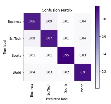
2.4 Evaluate Network Performance
Here, we have evaluated the performance of our network by calculating accuracy, classification report (precision, recall, and f1-score per class) and confusion matrix metrics on test predictions. We can notice from the results of metrics that our model seems to be doing a good job with good accuracy.
We have calculated various metrics using functions available from scikit-learn. Please feel free to check the below link if you are interested in learning about various metrics available from sklearn in detail.
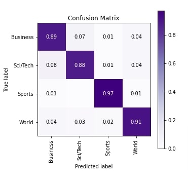
In the next cell after the below cell, we have also plotted the confusion matrix using the function available from scikit-plot python library. We can notice from the plots that our model is doing good for categories Sports and World compared to categories Business and Sci/Tech. Please feel free to check the below link if you want to learn scikit-plot libraries which provide visualization for many ML metrics.
from sklearn.metrics import accuracy_score, classification_report, confusion_matrix

train_preds = model.apply(final_weights, X_train_vect)
test_preds = model.apply(final_weights, X_test_vect)

print("Train Accuracy : {:.3f}".format(accuracy_score(Y_train, np.argmax(train_preds, axis=1))))
print("Test  Accuracy : {:.3f}".format(accuracy_score(Y_test, np.argmax(test_preds, axis=1))))
print("\nClassification Report : ")
print(classification_report(Y_test, np.argmax(test_preds, axis=1), target_names=target_classes))
print("\nConfusion Matrix : ")
print(confusion_matrix(Y_test, np.argmax(test_preds, axis=1)))
from sklearn.metrics import confusion_matrix
import scikitplot as skplt
import matplotlib.pyplot as plt

skplt.metrics.plot_confusion_matrix([target_classes[i] for i in Y_test], [target_classes[i] for i in np.argmax(test_preds, axis=1)],
                                    normalize=True,
                                    title="Confusion Matrix",
                                    cmap="Purples",
                                    hide_zeros=True,
                                    figsize=(5,5)
                                    );
plt.xticks(rotation=90);
2.5 Explain Network Predictions Using LIME
In this section, we have tried to explain predictions made by the network using LIME algorithm. The lime python library provides an implementation of LIME algorithm. In order to use it, we first need to create an instance of LimeTextExplainer object and call explain_instance() method on it to generate Explanation object. The Explanation object has details about which words contributed to predicting a particular category. We can call show_in_notebook() method on Explanation object to generate visualization showing words contribution to prediction. Please feel free to check the below tutorial if you do not have a background on LIME and are interested in learning it.
Below, we have created an instance of LimeTextExplainer by giving target labels to it.
from lime import lime_text

explainer = lime_text.LimeTextExplainer(class_names=target_classes, verbose=True)
Below, we have designed a simple function that takes an input list of text documents and returns predictions for them. The function takes a list of text documents and converts them to a list of indexes using our trained tokenizer from earlier. It then gives this list of indexes to the network to make predictions. The prediction of the network is converted to probabilities using softmax activation function before returning from the function.
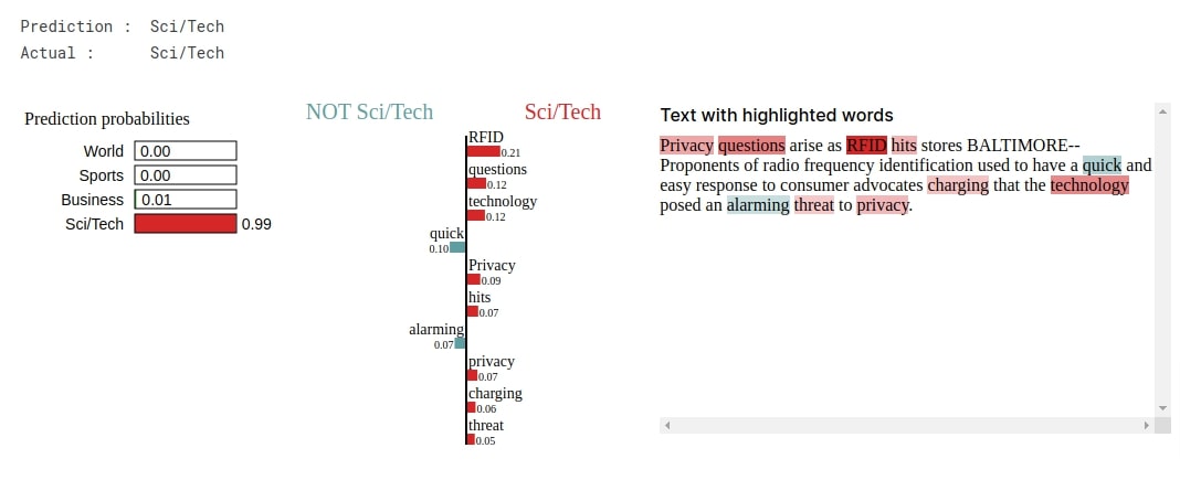
After defining a function, we have randomly selected a text sample from test data. We have then made predictions on it using our model. We have printed the actual label and predicted label for the selected sample. The actual label for our selected sample is Sci/Tech and our model predicted the same.
import numpy as np

def make_predictions(X_batch_text):
    X_batch = pad_sequences(tokenizer.texts_to_sequences(X_batch_text), maxlen=50, padding="post", truncating="post", value=0.)
    logits = model.apply(final_weights, jnp.array(X_batch))
    preds = linen.softmax(logits)
    return preds.to_py()

rng = np.random.RandomState(1234)
idx = rng.randint(1, len(X_test_text))

print("Prediction : ", target_classes[model.apply(final_weights, X_test_vect[idx:idx+1]).argmax(axis=-1)[0]])
print("Actual :     ", target_classes[Y_test[idx]])
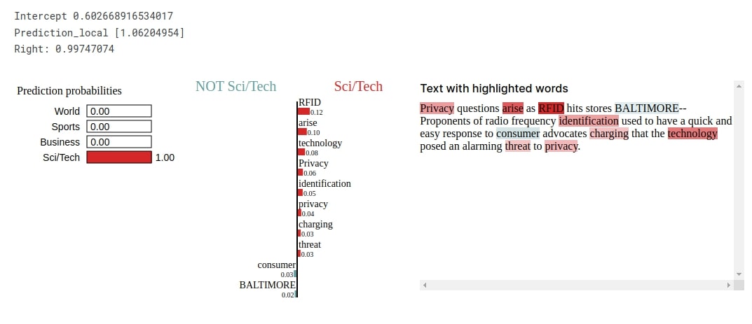
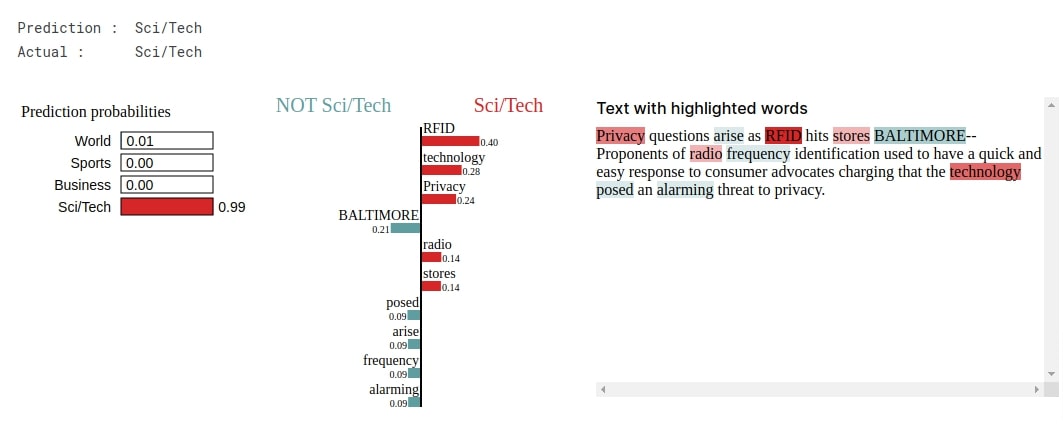
Below, we have called explain_instance() method on explain objects with the selected sample, classifier function (the one we defined in the previous cell), and actual label that we want to explain. The method returns an Explanation object. Then, we have called show_in_notebook() method on Explanation instance to create a visualization.
We can notice from the visualization that words like 'RFID', 'frequency', 'identification', 'technology', 'threat', 'privacy', etc are contributing to predicting category as Sci/Tech.
explanation = explainer.explain_instance(X_test_text[idx], classifier_fn=make_predictions, labels=Y_test[idx:idx+1].to_py())
explanation.show_in_notebook()
3. Approach 2 - Word Embeddings With More Values 
In this section, we have tried another approach to explaining word embeddings. Our approach for this section is exactly the same as our previous approach with only differences in embedding size. In this section, we have used an embedding size of 20 which is more compared to the previous example. The majority of the code in this section is the same as our code from the previous section with only a change in embedding length per word/token.
3.1 Define Network
Below, we have defined the network that we'll use for classification. The network has the exactly same structure as our previous network with only a difference in embedding length defined when creating the embedding layer. We have set it to 20 this time.
from flax import linen

class EmbeddingClassifier(linen.Module):
    def setup(self):
        self.embedding = linen.Embed(len(tokenizer.word_index)+1, 20, name="Word Embeddings") ## Word embeddings size increased
        self.linear1 = linen.Dense(100, name="Dense1")
        self.linear2 = linen.Dense(len(unique_classes), name="Dense2")

    def __call__(self, X_batch):
        x = self.embedding(X_batch)
        x = x.reshape(len(X_batch), -1)

        x = self.linear1(x)
        x = linen.relu(x)

        logits = self.linear2(x)
        return logits
3.2 Train Network
Now, we have trained our new network with more embeddings. We have initialized batch size to 1024, a number of epochs to 1024, and the learning rate to 0.001. Then, we have initialized our network and Adam optimizer. At last, we have called our training routine to perform training. We can notice from the training loss and validation accuracy that our model is doing a good job.
from jax import random

seed = random.PRNGKey(0)
batch_size=1024
epochs=15
learning_rate = jnp.array(1e-3)

model = EmbeddingClassifier()
params = model.init(seed, X_train_vect[:5])

optimizer = optax.adam(learning_rate=learning_rate)
optimizer_state = optimizer.init(params)

final_weights = TrainModelInBatches(X_train_vect, Y_train, X_test_vect, Y_test, epochs, params, optimizer_state, batch_size=batch_size)
3.3 Evaluate Network Performance
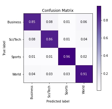
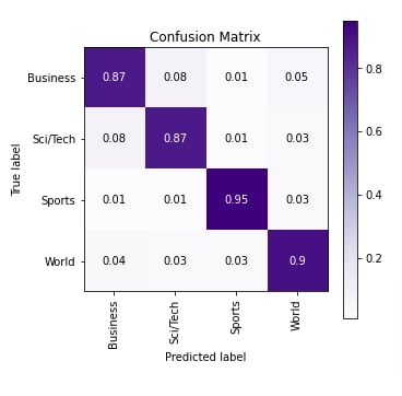
Here, we have calculated accuracy, classification report and confusion matrix metrics for test predictions. We can notice from the accuracy that it is almost the same as our accuracy from the previous section. The increase in embedding length does not seem to have increased accuracy much. The results of other metrics are almost the same with little to no improvements.
from sklearn.metrics import accuracy_score, classification_report, confusion_matrix

train_preds = model.apply(final_weights, X_train_vect)
test_preds = model.apply(final_weights, X_test_vect)

print("Train Accuracy : {:.3f}".format(accuracy_score(Y_train, np.argmax(train_preds, axis=1))))
print("Test  Accuracy : {:.3f}".format(accuracy_score(Y_test, np.argmax(test_preds, axis=1))))
print("\nClassification Report : ")
print(classification_report(Y_test, np.argmax(test_preds, axis=1), target_names=target_classes))
print("\nConfusion Matrix : ")
print(confusion_matrix(Y_test, np.argmax(test_preds, axis=1)))
from sklearn.metrics import confusion_matrix
import scikitplot as skplt
import matplotlib.pyplot as plt

skplt.metrics.plot_confusion_matrix([target_classes[i] for i in Y_test], [target_classes[i] for i in np.argmax(test_preds, axis=1)],
                                    normalize=True,
                                    title="Confusion Matrix",
                                    cmap="Purples",
                                    hide_zeros=True,
                                    figsize=(5,5)
                                    );
plt.xticks(rotation=90);
3.4 Explain Network Predictions Using LIME
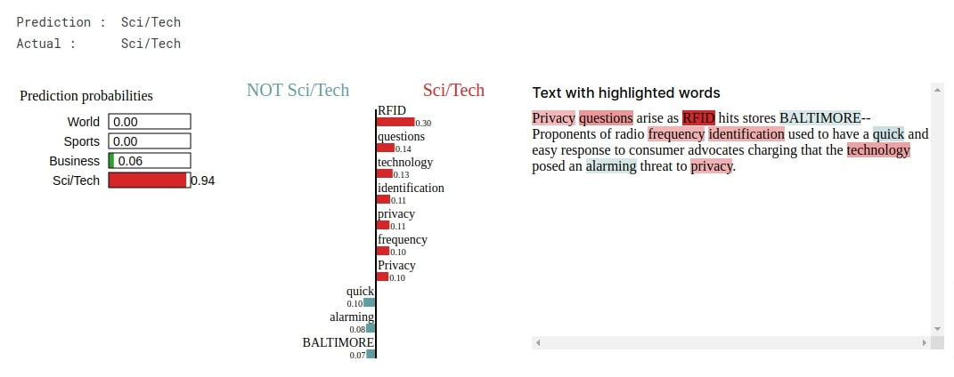
Below, we have again tried to explain the prediction made by the network. We have randomly selected a test example. The selected sample has Sci/Tech label and the network predicted the same. We can notice from the visualization that this time few words ('frequency', 'identification', 'threat', etc) that were contributing to prediction in the previous section are not contributing anymore.
from lime import lime_text

explainer = lime_text.LimeTextExplainer(class_names=target_classes)

rng = np.random.RandomState(1234)
idx = rng.randint(1, len(X_test_text))

print("Prediction : ", target_classes[model.apply(final_weights, X_test_vect[idx:idx+1]).argmax(axis=-1)[0]])
print("Actual :     ", target_classes[Y_test[idx]])

explanation = explainer.explain_instance(X_test_text[idx], classifier_fn=make_predictions, labels=Y_test[idx:idx+1].to_py())
explanation.show_in_notebook()
4. Approach 3 - Word Embeddings Averaged 
In this section, we have tried another approach involving word embeddings. We have used an embedding length of 20 like our previous section. The only difference in this approach is that, till now, we were flattening the embeddings but this time we have averaged embeddings of all words/tokens per text example. The averaged embedding is then given to dense layers.
4.1 Define Network
Our network for this section is exactly the same as our network from the previous section. The only difference is in the implementation of the forward pass. In this section, we have averaged the output of the embedding layer before giving it to the linear layer. We have averaged it in a way that word embeddings for a single text example will be averaged. As we have kept 50 tokens/words per text example, the network will average embeddings of all 50 tokens/words.
from flax import linen

class EmbeddingClassifier(linen.Module):
    def setup(self):
        self.embedding = linen.Embed(len(tokenizer.word_index)+1, 20, name="Word Embeddings")
        self.linear1 = linen.Dense(100, name="Dense1")
        self.linear2 = linen.Dense(len(unique_classes), name="Dense2")

    def __call__(self, X_batch):
        x = self.embedding(X_batch)
        x = x.mean(axis=1) ## Average word embeddings for each words together

        x = self.linear1(x)
        x = linen.relu(x)

        logits = self.linear2(x)
        return logits
4.2 Train Network
Below, we have trained our network using exactly the same settings that we have used in our previous sections. The training loss and validation accuracy printed at the end of the epoch points out that our model seems to be doing quite a good job compared to previous approaches we tried.
from jax import random

seed = random.PRNGKey(0)
batch_size=1024
epochs=15
learning_rate = jnp.array(1e-3)

model = EmbeddingClassifier()
params = model.init(seed, X_train_vect[:5])

optimizer = optax.adam(learning_rate=learning_rate)
optimizer_state = optimizer.init(params)

final_weights = TrainModelInBatches(X_train_vect, Y_train, X_test_vect, Y_test, epochs, params, optimizer_state, batch_size=batch_size)
4.3 Evaluate Network Performance
Below, we have calculated accuracy, classification report and confusion matrix metrics on test predictions as usual. We can notice from the accuracy that it's better than both of our previous approaches. The model's accuracy in classifying text documents from Business and Sci/Tech has increased compared to previous approaches.
from sklearn.metrics import accuracy_score, classification_report, confusion_matrix

train_preds = model.apply(final_weights, X_train_vect)
test_preds = model.apply(final_weights, X_test_vect)

print("Train Accuracy : {:.3f}".format(accuracy_score(Y_train, np.argmax(train_preds, axis=1))))
print("Test  Accuracy : {:.3f}".format(accuracy_score(Y_test, np.argmax(test_preds, axis=1))))
print("\nClassification Report : ")
print(classification_report(Y_test, np.argmax(test_preds, axis=1), target_names=target_classes))
print("\nConfusion Matrix : ")
print(confusion_matrix(Y_test, np.argmax(test_preds, axis=1)))
from sklearn.metrics import confusion_matrix
import scikitplot as skplt
import matplotlib.pyplot as plt

skplt.metrics.plot_confusion_matrix([target_classes[i] for i in Y_test], [target_classes[i] for i in np.argmax(test_preds, axis=1)],
                                    normalize=True,
                                    title="Confusion Matrix",
                                    cmap="Purples",
                                    hide_zeros=True,
                                    figsize=(5,5)
                                    );
plt.xticks(rotation=90);
4.4 Explain Network Predictions Using LIME
Below, we have explained one test prediction using LIME. We can notice from the visualization that words like 'privacy', 'RFID', 'frequency', 'technology', etc are contributing to predicting the category Sci/Tech.
from lime import lime_text

explainer = lime_text.LimeTextExplainer(class_names=target_classes)

rng = np.random.RandomState(1234)
idx = rng.randint(1, len(X_test_text))

print("Prediction : ", target_classes[model.apply(final_weights, X_test_vect[idx:idx+1]).argmax(axis=-1)[0]])
print("Actual :     ", target_classes[Y_test[idx]])

explanation = explainer.explain_instance(X_test_text[idx], classifier_fn=make_predictions, labels=Y_test[idx:idx+1].to_py())
explanation.show_in_notebook()
5. Approach 4 - Word Embeddings Summed 
Our approach in this section has the majority of the code same as our previous approach with the only difference that we are summing up embeddings for text examples instead of averaging them this time.
5.1 Define Network
Below, we have defined our network which has the almost same structure as our network from the previous approach. The only difference is in the forward pass of the network. We are summing up embeddings of text examples this time instead of averaging.
from flax import linen

class EmbeddingClassifier(linen.Module):
    def setup(self):
        self.embedding = linen.Embed(len(tokenizer.word_index)+1, 20, name="Word Embeddings")
        self.linear1 = linen.Dense(100, name="Dense1")
        self.linear2 = linen.Dense(len(unique_classes), name="Dense2")

    def __call__(self, X_batch):
        x = self.embedding(X_batch)
        x = x.sum(axis=1) ## Sum word embeddings for each words together

        x = self.linear1(x)
        x = linen.relu(x)

        logits = self.linear2(x)
        return logits
5.2 Train Network
Below, we have trained our network using the same settings that we have been using for all our previous approaches. We can notice from the loss and accuracy getting printed after each epoch that our model has done a good job at the text classification task.
from jax import random

seed = random.PRNGKey(0)
batch_size=1024
epochs=15
learning_rate = jnp.array(1e-3)

model = EmbeddingClassifier()
params = model.init(seed, X_train_vect[:5])

optimizer = optax.adam(learning_rate=learning_rate)
optimizer_state = optimizer.init(params)

final_weights = TrainModelInBatches(X_train_vect, Y_train, X_test_vect, Y_test, epochs, params, optimizer_state, batch_size=batch_size)
5.3 Evaluate Network Performance
Below, we have evaluated network performance as usual by calculating accuracy, classification report and confusion matrix metrics on test predictions. The accuracy is pretty good for this model as well.
from sklearn.metrics import accuracy_score, classification_report, confusion_matrix

train_preds = model.apply(final_weights, X_train_vect)
test_preds = model.apply(final_weights, X_test_vect)

print("Train Accuracy : {:.3f}".format(accuracy_score(Y_train, np.argmax(train_preds, axis=1))))
print("Test  Accuracy : {:.3f}".format(accuracy_score(Y_test, np.argmax(test_preds, axis=1))))
print("\nClassification Report : ")
print(classification_report(Y_test, np.argmax(test_preds, axis=1), target_names=target_classes))
print("\nConfusion Matrix : ")
print(confusion_matrix(Y_test, np.argmax(test_preds, axis=1)))
from sklearn.metrics import confusion_matrix
import scikitplot as skplt
import matplotlib.pyplot as plt

skplt.metrics.plot_confusion_matrix([target_classes[i] for i in Y_test], [target_classes[i] for i in np.argmax(test_preds, axis=1)],
                                    normalize=True,
                                    title="Confusion Matrix",
                                    cmap="Purples",
                                    hide_zeros=True,
                                    figsize=(5,5)
                                    );
plt.xticks(rotation=90);
5.4 Explain Network Predictions Using LIME
Here, we have explained the prediction made by our model on a random test example using LIME. The network correctly predicts the category as 'Sci/Tech' for the selected sample. The visualization shows that words like 'privacy', 'RFID', 'charging', 'technology', 'threat', etc are contributing to predicting category 'Sci/Tech'.
from lime import lime_text

explainer = lime_text.LimeTextExplainer(class_names=target_classes)

rng = np.random.RandomState(1234)
idx = rng.randint(1, len(X_test_text))

print("Prediction : ", target_classes[model.apply(final_weights, X_test_vect[idx:idx+1]).argmax(axis=-1)[0]])
print("Actual :     ", target_classes[Y_test[idx]])

explanation = explainer.explain_instance(X_test_text[idx], classifier_fn=make_predictions, labels=Y_test[idx:idx+1].to_py())
explanation.show_in_notebook()
This ends our small tutorial explaining how we can use word embeddings for Flax (JAX) text classification networks. Please feel free to let us know your views in the comments section.
References
 Sunny Solanki
Sunny Solanki
Intro: Software Developer | Youtuber | Bonsai Enthusiast
About: Sunny Solanki holds a bachelor's degree in Information Technology (2006-2010) from L.D. College of Engineering. Post completion of his graduation, he has 8.5+ years of experience (2011-2019) in the IT Industry (TCS). His IT experience involves working on Python & Java Projects with US/Canada banking clients. Since 2020, he’s primarily concentrating on growing CoderzColumn.
His main areas of interest are AI, Machine Learning, Data Visualization, and Concurrent Programming. He has good hands-on with Python and its ecosystem libraries.
Apart from his tech life, he prefers reading biographies and autobiographies. And yes, he spends his leisure time taking care of his plants and a few pre-Bonsai trees.
Contact: sunny.2309@yahoo.in


![YouTube Subscribe]() Comfortable Learning through Video Tutorials?
Comfortable Learning through Video Tutorials?
If you are more comfortable learning through video tutorials then we would recommend that you subscribe to our YouTube channel.
![Need Help]() Stuck Somewhere? Need Help with Coding? Have Doubts About the Topic/Code?
Stuck Somewhere? Need Help with Coding? Have Doubts About the Topic/Code?
 Stuck Somewhere? Need Help with Coding? Have Doubts About the Topic/Code?
When going through coding examples, it's quite common to have doubts and errors.
If you have doubts about some code examples or are stuck somewhere when trying our code, send us an email at coderzcolumn07@gmail.com. We'll help you or point you in the direction where you can find a solution to your problem.
You can even send us a mail if you are trying something new and need guidance regarding coding. We'll try to respond as soon as possible.
![Share Views]() Want to Share Your Views? Have Any Suggestions?
Want to Share Your Views? Have Any Suggestions?
 Want to Share Your Views? Have Any Suggestions?
If you want to
- provide some suggestions on topic
- share your views
- include some details in tutorial
- suggest some new topics on which we should create tutorials/blogs
 flax, jax, word-embeddings, text-classification