Guide to Text Generation using MXNet RNNs (LSTM) (Character Embeddings)¶

Text generation is a type of language modeling task where we create a language model to generate new text. It is an active area of research under NLP. These language model needs to understand the structure of language (grammar, spellings, etc) in order to generate new text. The language models like these are used for tasks like text translation, conversational systems (chatbots), speech-to-text, text summarization, etc. Nowadays deep neural networks are getting developed for text generation tasks. The commonly used architecture for text generation tasks is Recurrent Neural Networks (RNNs). The RNNs and their variants (LSTM, GRU, etc) are quite good at remembering sequences in data. As with text generation tasks also, we need it to understand the sequence of words/characters in order to predict new words/characters, these models are quite a good choice.

As a part of this tutorial, we'll explain how we can create Recurrent Neural Networks (RNNs) consisting of LSTM Layers using Python Deep Learning library MXNet for solving text generation task. We'll be using character-based approach for text generation where we'll give network a few characters and will ask it to generate a new character after those characters. To encode text, we'll combine bag of words with character embeddings. We have used Wikipedia dataset available from torchtext to train our network. It has a list of well-curated Wikipedia articles. Apart from this one, we have one more tutorial on text generation using MXNet where we haven't used character embeddings to encode data. We have only used a bag of words. Please feel free to check the below link if it interests you.

• MXNet: Text Generation using LSTM (Character-based RNNs)

Below, we have listed important sections of the Tutorial to give an overview of the material covered.

Important Sections Of Tutorial¶

1. Prepare Data
   • 1.1 Load Data
   • 1.2 Populate Vocabulary
   • 1.3 Organize Data for Task
   • 1.4 Create Data Loader
2. Define Network
3. Train Network
4. Generate Text
5. Train Network More
6. Generate Text
7. Train Even More
8. Generate Text
9. Further Suggestions

Below, we have imported the necessary Python libraries and printed the versions that we have used in our tutorial.

1. Prepare Data ¶

In this section, we are preparing data that will be given to network for training purposes. We have decided that we'll be giving network 100 characters and ask it to predict the next character after those characters. As explained earlier, we'll be using character embeddings as our encoding method. We'll be following the below steps to prepare data.

1. Load Data
2. Loop through each text example of data and create a vocabulary of unique characters. A vocabulary is a simple mapping from a character to an integer index. Each character is assigned a unique integer index starting from 0.
3. Move the window of size 100 through the text of each text example taking characters inside the window as data features (X) and a character coming after the window as the target value (Y). To explain with an example,
   • Characters 1-100 will be data features (X) and character 101 will be the target value (Y).
   • Move the window by 1 position.
   • Characters 2-101 will be data features (X) and character 102 will be target value (Y).
   • Move the window by 1 position.
   • Characters 3-102 will be data features (X) and character 103 will be target value (Y).
   • and so on.
4. Retrieve integer indexing for characters present in data features (X) and target values (Y) using our populated vocabulary. After completion of this step, data features (X) and target values (Y) will be arrays of integers.
5. Assign a real-valued vector (character embeddings) to each integer of data features (X). This step will be performed by embedding layer of the neural network.

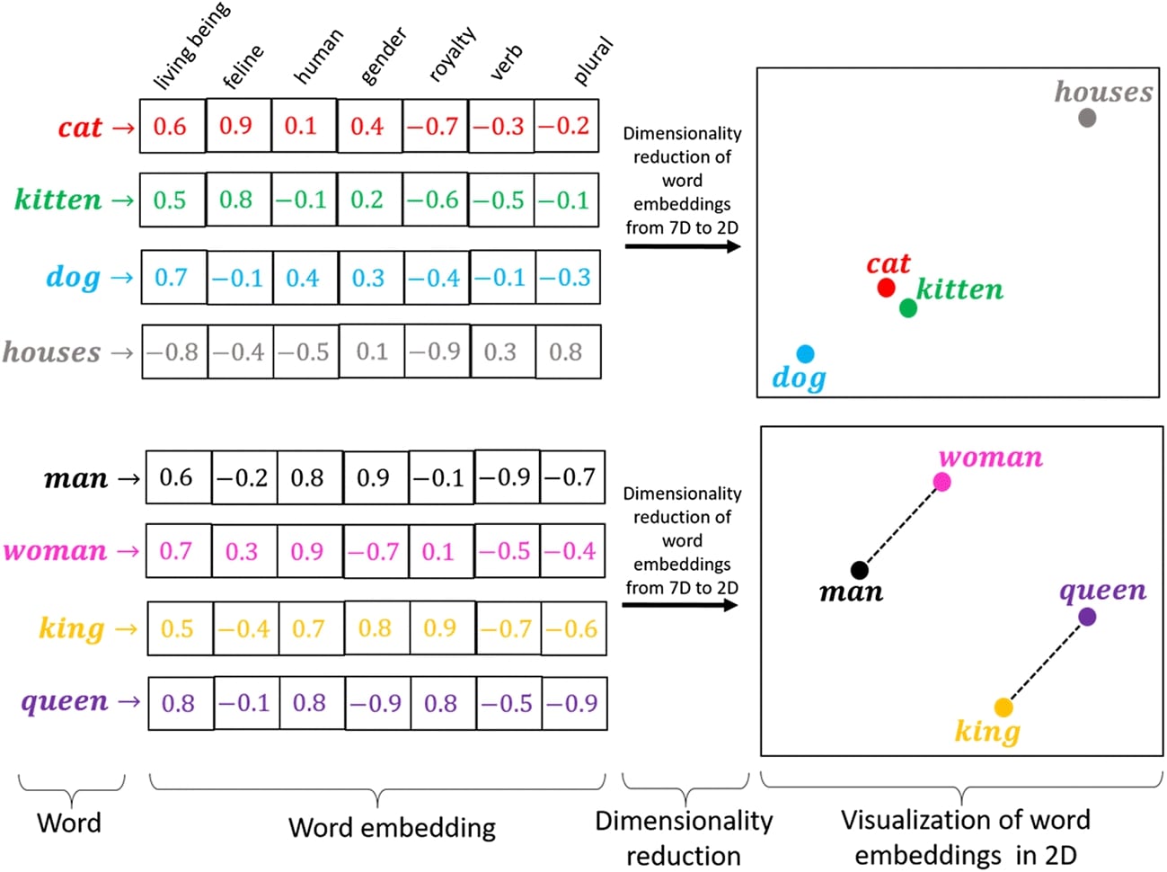
In short, we'll first map characters to integer indexes and then will map integer indexes to character embeddings. The steps till mapping to integer indexes will be performed in this section. The mapping of an integer index to its character embedding (real-valued vector) will be performed by the embedding layer of the network. The embedding is a real-valued vector assigned to a character (through integer index mapping) which will give it more representation power.

Below, we have included an image that shows word embeddings. The character embedding is almost same with the only difference being that we are assigning a real-valued vector to an individual character.

1.1 Load Data¶

In this section, we have simply loaded Wikipedia dataset that we are going to use for our case. The dataset has well-curated Wikipedia articles. The dataset is available from torchtext library. It is already divided into train, validation, and test sets. We'll be using the train set for our purposes which have ~36k text documents.

1.2 Populate Vocabulary¶

In this section, we are populating the vocabulary of unique characters. To populate vocabulary, we have used count_tokens() helper function available from gluonnlp library of mxnet. The method takes as an input list of characters and Counter object. It then updates the count of characters present in the list of characters to Counter object. The Counter object is available from Python collections module. It let us maintain the count of keys. We have initially created an empty Counter object. We are then looping through each text example of the train dataset calling count_tokens() method on the list of characters of text examples. Each call to count_tokens() updates Counter object with count of characters present in that example. After completion of the loop, the Counter object will have a count of each character present in the train dataset. We can then create vocabulary by calling Vocab() constructor with Counter object.

After the creation of vocabulary, we have printed vocabulary content and its size as well. We can see how each character is assigned a unique integer index.

1.3 Organize Data for Task¶

In this section, we are organizing our data for the neural network. We have set sequence length as 100 characters as discussed earlier. We'll be giving 100 characters to network and make it predict the next character after them.

In order to prepare data for training, we are looping through text examples of train dataset moving window of size 100 through them. We are adding character that falls inside a window in data features (X_train) and the next character after them in target values (Y_train). Then, we are retrieving integer indexes of characters present in data features (X_train) and target values (Y_train) using our populated vocabulary. After completion of the loop, we'll have two arrays (X_train, Y_train) which will have integer indexes present in them. We have converted these arrays to mxnet nd arrays as required by MXNet networks.

Please make a note that we have not used all text documents present inside of the train dataset as it'll take a lot of training time.

Below we have explained with a simple example how the process works.

vocab = {
'h':1,
'e':2,
'l':3,
'o':4,
' ':5,
',':6,
'w',7,
'a':8,
'r':9,
'y':10,
'u':11,
'?':12,
'c':13,
'm':14,
't':15,
'd':16,
'z':17,
'n':18
}

text_example = "Hello, How are you? Welcome to coderzcolumn?"
seq_length = 10

X_train = [
            ['h','e','l','l','o',',',' ', 'h','o','w'],
            [,'e','l','l','o',',',' ', 'h','o','w',' '],
            ['l','l','o',',',' ', 'h','o','w', ' ', 'a'],
            ['l','o',',',' ', 'h','o','w',' ', 'a', 'r'],
            ...
            ['d','e','r','z','c','o','l', 'u','m','n']
            ]
Y_train = ['e','l','l','o',',',' ', 'h','o','w',' ',..., '?']

X_train_vectorized = [
                        [1,2,3,4,5,6,1,4,7],
                        [2,3,4,5,6,1,4,7,5],
                        [3,4,5,6,1,4,7,5,1],
                        ...
                        [16,2,9,17,13,4,3,11,14,18]
                     ]
Y_train_vectorized = [1,2,3,4,5,6,1,4,7,5,1,...., 12]

1.4 Create Data Loader¶

In this section, we have simply wrapped nd arrays (X_train, Y_train) inside ArrayDataset and then created a data loader from the dataset object. This data loader object will let us loop through training data easily in batches. We have set the batch size to 1024. We have also set shuffle argument to False as we don't want to disturb the character sequence.

2. Define Network ¶

In this section, we have defined a network that we'll use for our task. Our task will be a classification task as we'll be predicting one of the vocabulary character indexes. The network consists of 4 layers.

1. Emebdding Layer
2. LSTM Layer
3. LSTM Layer
4. Dense Layer

The first layer of our network is the embedding layer which we have created using Embedding() constructor available from "nn" sub-module of MXnet. We have provided vocabulary length and embedding length to the constructor. The embedding length in our case is 50 which means that each character index will be assigned a real-valued vector of length 50. This constructor will create an integer weight matrix of shape (vocab_len, embedding_len). For each character index, the real-valued vector (embedding) will be retrieved by simply integer indexing this weight matrix. The input shape to embedding layer is (batch_size, seq_len) = (batch_size, 100) and output data shape is (batch_size, seq_len, embed_len) = (batch_size, 100, 50).

The output of the embedding layer is given to the first LSTM layers for processing. We have created LSTM layers using LSTM() constructor. The hidden size of the LSTM layer is set as 256 and num_layers parameter is set as 2 instructing the constructor to stack two LSTM layers. The first LSTM layer will transform data from shape (batch_size, 100, 50) to (batch_size, 100, 256). The output of the first LSTM layer will be given to the second LSTM layer which has the same output shape as the first LSTM layer.

The output of the second LSTM layer is given to a dense layer for the processing which has the same output units as the number of characters in vocabulary because we want it to predict the next character. The output of the dense layer is a prediction of our network

After defining the network, we initialized it, made predictions with random data for verification, and printed the shape of weight/biases of each layer.

Please make a NOTE that we have not discussed LSTM layers in detail in this tutorial as we have assumed that the reader has background on it. If you want to know about LSTM then we recommend that you go through the below tutorial which covers it in detail. It can help you with this tutorial.

• MXNet: LSTM Networks for Text Classification Tasks

If you are new to MXNet and want to learn how to create neural networks using it then we suggest that you go through the below tutorial.

• Simple Guide to Create Neural Networks using MXNet

3. Train Network ¶

In this section, we are training our network. To train the network, we have designed a simple function that will let us perform the training process. The function takes Trainer* object (network parameters), train data loader, and a number of epochs as input. It executes a training loop number of epochs time. During each epoch, it loops through training data in batches using a train data loader. During each batch, it performs a forward pass to make predictions, calculates loss, calculates gradients, and updates network parameters. The loss for each batch is recorded and an average loss of all batches per epoch is printed at the end of an epoch.

Below, we are actually training our network using the training routine defined in the previous cell. We have initialized a number of epochs to 50 and the learning rate to 0.001. Then, we have initialized our model, cross-entropy loss function, Adam optimizer, and Trainer object. The trainer object holds network parameters and will be responsible for updating them after each forward pass. At last, we have called our training routine with the necessary parameters to perform the training process.

We can notice from the loss value getting printed after epochs that our network seems to be doing a good job at the task as loss is decreasing constantly.

4. Generate Text ¶

In this section, we are generating text using our trained network to see how it is performing. We have randomly selected a 100 characters sequence from the train data we prepared earlier. Then we generated 100 characters after them using our trained network using a loop. During the first iteration of the loop, we give the selected sequence as input to network to predict the next character. The output character index of the first iteration is appended at the end of our sequence and the first index is removed from the sequence. This is done to keep the length of sequence consistent at 100. For the second iteration, this modified sequence of character indexes will be given to the network to make a prediction of the next character. The output of the second iteration is appended at the end of the sequence and the first character is removed from the sequence. This modified sequence becomes the input of the model for the third iteration. This process is repeated for all iterations. In the end, the generated 100 characters are printed.

We can see that generated text seems like English language text though it is not making any sense. The model is properly spelling words. It is also able to generate punctuation marks. Overall the result is good. We'll train the network further to see whether it is improving results further or not.

5. Train Network More ¶

In this section, we are training the network for another 50 epochs with a learning rate of 0.0003. We can notice from the loss values getting printed that they are decreasing which is a sign of improvement. Next, we'll check the performance of the network by generating new text.

6. Generate Text ¶

In this section, we have again generated text using our network which is trained for 50 more epochs now. The code to generate text is exactly the same as earlier. We have started with the same text sequence which we used earlier when generating text. The text generated by the network seems satisfactory though it is not making much sense it looks like English language text. The model is generating proper words this time as well. We'll further train the network to see whether it is further improving.

7. Train Even More ¶

In this section, we have trained the network for another 50 epochs with a learning rate of 0.0001. We can notice from the loss values that the network seems to be improving. We'll check the performance next by generating text.

8. Generate Text ¶

In this section, we have generated text using our network. We have used the same code to generate text that we have been using for all previous text generations. We can notice that network is properly generating text. The text generated still does not make much sense but looks like English language text. The words are correctly spelled. Next, we have given a few suggestions on how network performance can be improved further.

9. Further Suggestions ¶

1. Train the network for more epochs.
2. Try different sequence lengths. We used a sequence length of 100 characters.
3. Try to generate more next characters. We had generated just one next character.
4. Try different LSTM output sizes.
5. Add more LSTM layers. This can increase training time drastically hence think thrice before trying.
6. Try the n-gram/word-based model instead of the character-based.
7. Try learning rate schedulers
8. Add little randomness to the prediction of the next character. REFERENCE

References¶

• MXNet: LSTM Networks for Text Classification Tasks
• Simple Guide to Create Neural Networks using MXNet