Keras: Guide to Create Simple Neural Networks in Python¶

Traditional ML models (linear regression, logistic regression, decision trees, random forests, gradient boosting machines, etc) are quite good at solving tasks involving structured datasets (tabular data). Over time these models were even tried on unstructured datasets (text, image, audio, etc) but the results were not that impressive.

Various research showed that deep neural networks consisting of many layers of different types (dense, convolution, recurrent, etc.) are quite good at handling unstructured datasets.

This gave rise to the whole new field of deep learning which primarily concentrates on creating deep neural networks to solve tasks.

Over the years, many Python libraries (Keras, PyTorch, Tensorflow, Theano, MXNet, JAX, Haiku, Flax, etc) were created to create neural networks. All these libraries offer simple APIs to create and train neural networks faster.

What can you learn from this article?¶

As a part of this tutorial, we have explained how to create neural networks using Python library Keras which is now available through Python library Tensorflow. The tutorial explains how we can create simple neural networks using sequential API and functional API of Keras. We have created neural networks to solve classification and regression tasks on toy datasets available from scikit-learn.

The whole flow of ML tasks starting from downloading the dataset, creating the model, training the model, and evaluating performance (by calculating ML metrics) is covered.

This tutorial is a very good starting point for someone who is new to keras library. It'll make you aware of basic API within an hour.

Below, we have listed important sections of the Tutorial to give an overview of the material covered.

Important Sections Of Tutorial¶

1. Regression
   • 1.1 Load Dataset
   • 1.2 Normalize Data
   • 1.3 Create Neural Network Regressor using "Sequential()" or "Model()"
     • Sequential API
     • Functional API
   • 1.4 Compile Neural Network using "compile()"
   • 1.5 Train Neural Network using "fit()"
   • 1.6 Make Predictions using "predict()"
   • 1.7 Evaluate Performance using "evaluate()"
2. Classification
   • Same sub-sections as regression section

Below, we have imported the necessary Python libraries that we have used in our tutorial and printed the versions as well.

1. Regression ¶

In this section, we have explained how we can create simple neural networks using Keras to solve regression tasks. We have used Boston housing dataset available from scikit-learn for our purpose. We'll use a neural network to predict house prices using other data features of the house.

1.1 Load Dataset¶

Her, we have loaded Boston housing dataset available from scikit-learn. The dataset has 13 features of houses like number of bedrooms, crime rate in area, etc. The target value is a median value of a house in 1000's dollars. The dataset is loaded using load_boston() method of datasets module.

After loading dataset, the dataset is divided into train (80%) and test (20%) sets using train_test_split() function of scikit-learn.

1.2 Normalize Data¶

Here, we have normalized our train and test datasets to bring all columns of data in almost the same range. When we normalize data, there is less variance in column values. This helps the optimization algorithm to converge faster as a high difference in values of columns can give hard times to optimization algorithm. It can even prevent it from converging sometime.

To normalize data, we first calculated mean and standard deviation of each column of train data. Then, we subtracted mean from both datasets and divided subtracted values by standard deviation. This will help us get better results faster.

1.3 Create Neural Network Regressor using "Sequential()" or "Model()"¶

Here, we have explained different ways of creating a neural network using Keras. Currently, keras provides two different APIs for creating neural networks.

1. Sequential API - Here, we first create an instance of Sequential() object and add one by one layer (dense, convolution, max pooling, etc) to it. The network will process data in sequence as the layers are added to it. It won't let us create a complicated structure where we want to try something other than simple sequential execution (E.g., we want to take output of a few previous layers and add them.).
2. Functional API - Here, we work with layers like they are functions. We initialize layers and then process data by calling instance of a layer. This way of creating networks gives us flexibility as it opens a host of different architectures which we can't try with sequential API. Keras provides Model() class for functional API.

In the majority of the cases, Sequential API will be able to do tasks and you'll rarely need Functional API. The very complex architectures (like ResNet, MobileNet, etc.) working with unstructured data are generally designed using Functional API.

1.3.1 Sequential API¶

In this section, we have created our first neural network using Sequential API of Keras.

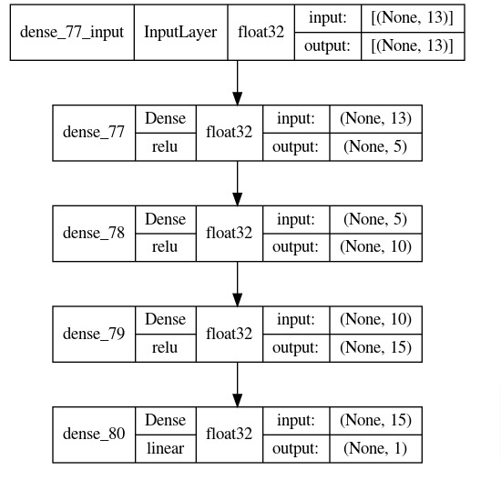
The network consists of 4 dense layers with output units 5, 10, 15, and 1 respectively. The first layer parameter input_shape is given a tuple specifying the shape of input data. The later layers will figure out shape by themselves. All first three layers apply relu (Rectified Linear Unit) activation to the output of layer. The relu function (relu(x) = max(0, x)) simply removes negative values and replaces them with 0s in processed data.

In order to create a network, we have initialized instance of Sequential from 'models' sub-module of Keras. Various layers are available from 'layers' sub-module. We have used Dense layer for our task.

When initializing Sequential object, we have given a list of layers inside it. The layers are created using Dense() constructor. The first argument to it is output units of that layer. The constructor has other parameters like activation, use_bias, kernel_initializer, activity_regularizer, etc.

The first layer will take input data with shape (batch_size, no_of_features) and transform it to shape (batch_size, 5) after processing. The second layer will transform output data from first layer to shape (batch_size, 10). The third layer will transform output data from first layer to shape (batch_size, 15). The fourth and last layer will transform data to shape (batch_size, 1) after processing which is an output of our network. The output of fourth layer is a prediction of our network.

After initializing network, we have printed a summary of output shapes and parameters count of individual layers. Then, in the next cell, we have also visualized model using Keras visualization util.

1.3.2 Sequential API¶

Here, we have explained one more way of creating a neural network using Sequential API. The network is almost same as earlier with only difference being that we have initialized Sequential instance first and then added layers to it one by one using add() method. This will create same network as we had given layers as a list to constructor.

1.3.3 Functional API¶

Here, we have created same neural network as or previous sections using Functional API.

First, we have created an instance of dense layers which we can call later. The layers are defined like previous sections only but are now stored in independent variables.

Then, we created an input layer using Input() constructor. This layer is just a placeholder declaring shape of input data. After defining input layer, we have called first layer with input layer. The output is stored in a variable which is given to second layer for processing and so on. The output from last layer is a prediction of network. Here, we called each layer to process input data hence this API is referred to as Functional API.

To create a model instance, we need to initialize Model object with input and output. In our case, the input will be input layer and output will be output object from last layer. When creating network like this we can also check shape of output layers for verification purposes to better understand layer processing.

After defining network, we have also printed a summary of shapes and parameters count of layers using summary() function.

1.4 Compile Neural Network using "compile()"¶

After defining Keras network, the next step is to compile it. The compilation step simply sets information like what optimizer, loss function, evaluation metrics, etc to use.

We can call compile() method on model object to compile models with necessary information. The optimizer, loss and metrics arguments accepts string as well as callable as input. We can give name of optimizer, loss function, and metrics to use for model. This will initialize them with default parameters. Keras let us also create an instance of optimizer (from 'keras.optimizers'), loss function (from 'keras.losses') and metrics (from 'keras.metrics') as well.

Though in a majority of situation providing string values that initializes these objects with default values will work well. You'll need to create an optimizer object, loss function, and metrics only when you need to try them with different values than default to improve results.

Below, we have compiled network to use 'sgd' (stochastic gradient descent) optimizer, 'mae' (mean absolute error) loss function and 'mse' (mean squared error) metric. The MAE and MSE are commonly used metrics for regression tasks.

1.5 Train Neural Network using "fit()"¶

Keras provides us with a method named fit() to train our network after it is compiled. This method will run only if it is called after compilation else it'll raise an error.

The fit method let us provide information below information through its parameters.

• x - Train data features. This can be a numpy array, tensorflow tensor, or keras generator object.
• y - Train target labels. This can be a numpy array or tensorflow tensor.
• batch_size - Batch size.
• epochs - Number of epochs.
• validation_data - Validation data. This accepts tuple of numpy arrays (x_val, y_val) or tensorflow tensors (x_val, y_val) specifying validation data. We can also give keras generator here.
• validation_split - Validation data percent from train data. If we don't want to provide validation data explicitly but want to use a fraction of train data for validation then we can provide a float value in the range 0-1 to this parameter. It'll take that much of train data as validation data. E.g., 0.2 will take 20% train data as validation data.
• shuffle - It accepts boolean values specifying whether to shuffle train data or not.
• callbacks - It accepts various callback functions that can be executed during various steps of training like before epoch, after completion of an epoch, etc. We have a detailed tutorial on Keras callbacks which we would recommend that readers go through in their free time.

The fit() method after completion returns a History object which has information about training process like values of train/Val loss and values of train/Val metrics after each epoch. The information is available through history parameter of History object as a dictionary.

Below, we have called fit() method twice (first time for 10 epochs and then for another 15 epochs) to train our network. We can notice that it prints loss and metric values after each epoch for both train and validation datasets.

1.6 Make Predictions using "predict()"¶

To make predictions, network provides us with predict() method. This method accepts data features as numpy array, tensorflow tensor, or keras generator object.

Below, we have made predictions on train and test datasets.

1.7 Evaluate Performance using "evaluate()"¶

We can evaluate the performance of network using evaluate() method. It'll calculate loss and metric values that were set when compiling network. We need to give data features (x) and target values (y) to evaluate network performance on them.

In our case, it returns MAE and MSE as set by us earlier during compilation step. We have evaluated network performance on both train and test datasets below.

We can also calculate metrics by calling metric function available from 'keras.metrics' module. We need to provide function actual target values and predicted values. We have calculated MSE using mse() function by providing actual target values and predicted values.

Apart from these ways, we can also use various metrics calculation functions available from scikit-learn. We have calculated r2 score for train and test predictions. It is a commonly used metric to evaluate performance of regression model and has a value in the range 0-1. The values near 1 are considered signs of a good generalized model.

If you are interested in learning about various models available from sklearn then we would recommend that you spend time on the below link.

• Scikit-learn: Model Evaluation and Scoring Metrics

2. Classification ¶

In this section, we have explained how to create a simple network using Keras to solve a classification task. We have used toy dataset available from scikit-learn for our purpose.

2.1 Load Dataset¶

Below, we have loaded Breast cancer dataset available from scikit-learn. The dataset has 30 features (independent variables). They are various measures of a tumor. The target variable is a binary telling us whether a tumor is benign (0) or malignant (1).

We have loaded dataset directly as numpy array by setting return_X_y parameter of load_breast_cancer() method to True.

After loading the dataset, we have divided it into train (80%) and test (20%) sets. We have printed the shapes of datasets for reference purposes. We have also stored number of features and classes in different variables as we'll need them later.

2.2 Normalize Data¶

Here, we have normalized our data like regression section. As explained earlier, this helps our optimization (SGD) algorithm to converge faster. We have used train data mean and standard deviation to normalize train and test datasets.

2.3 Create Neural Network Classifier¶

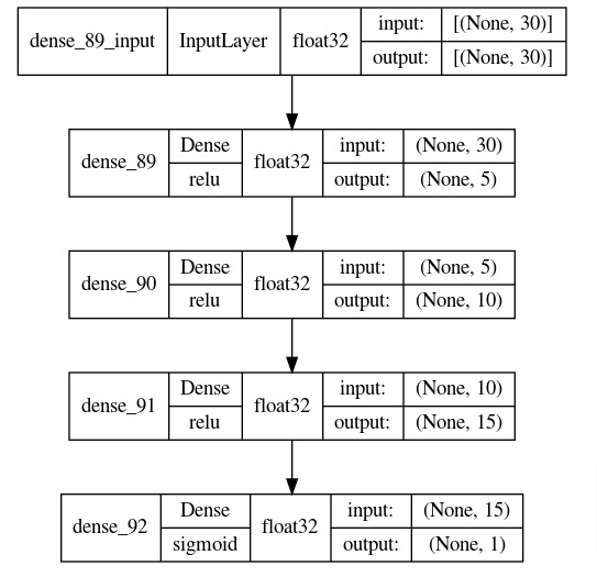
Here, we have created a network that we'll use for our classification task. The network consists of 4 dense layers like regression section. We have created a network using Sequential API of Keras.

The dense layers have 5, 10, 15, and 1 output units respectively. The first three layers have relu activation function whereas last layer has sigmoid activation function. The sigmoid activation function takes any input and transforms it into a float in the range 0-1. The output of last layer will be a prediction of our network which is an output of sigmoid function in this case.

After defining network, we have printed a summary of shapes and parameters count of layers. We have also plotted network using visualization util of Keras.

2.4 Compile Neural Network¶

Below, we have compiled our classification network to use SGD optimizer, binary cross entropy loss, and accuracy metric. As we have binary task of classifying tumors as malignant or benign, we have used binary cross entropy loss. The accuracy metric simply measures percentage of target labels that were correctly predicted by model.

2.5 Train Neural Network¶

In this section, we have trained our network by calling fit() method on model. We have trained network for 10 and 15 epochs respectively. The log messages show loss and accuracy metric values after each epoch. We can notice from these values that our network has improved after each epoch.

2.6 Make Predictions¶

Below, we have made predictions using our trained network by calling predict() method. We have made predictions on train and test datasets both. As we had explained earlier, the last layer of network is sigmoid function hence output of network will be in range 0-1.

Our actual target labels are binary (0 or 1). We can convert these probabilities to binary labels by setting a threshold at 0.5 and predicting label as 1 if a value is greater than 0.5 else 0 for less than 0.5.

2.7 Evaluate Performance¶

In this section, we have evaluated the performance of our classification network.

We have calculated loss and accuracy on both train and test datasets using evaluate() method. We can notice from the results that our model is doing a good job a the task.

We have also calculated loss and accuracy values separately using methods available from keras and sklearn for verification purposes.

Apart from accuracy, we have also calculated classification report metrics which have precision, recall, and f1-score per target class. It helps us better understand for which classes our model is doing a good job and for which class is not that good.

References¶

• Scikit-learn: Model Evaluation and Scoring Metrics