Scikit-Learn - Decision Trees
Table of Contents
- Introduction
- DecisionTreeClassifier
- ExtraTreeClassifier
- DecisionTreeRegressor
- ExtraTreeRegressor
- References
Introduction 
Decision Trees are a class of algorithms that are based on "if" and "else" conditions. Based on these conditions, decisions are made to the task at hand. These conditions are decided by an algorithm based on data at hand. How many conditions, kind of conditions, and answers to that conditions are based on data and will be different for each dataset. We'll be covering the usage of decision tree implementation available in scikit-learn for classification and regression tasks below.
Below we have highlighted some characteristics of decision tree
Characteristics of decision trees:
- Fast to train and easy to understand & interpret.
- Binary splitting of questions is the essence of decision tree models.
- Requires little preprocessing of data.
- Can work with variables of different types (continuous & discrete)
- Invariant to feature scaling.
- Models are called "nonparametric" because there are no hyper-parameters to tune.
- If given more data then the model becomes more flexible.
- Number of tree parameters (conditions) grows with the number of samples covering as much domain of data as possible.
We'll start by importing the necessary modules needed for our tutorial. We'll need pydotplus library installed as it'll be used to plot decision trees trained by scikit-learn.
## We need to install pydotplus for this tutorial.
!pip install pydotplus
import numpy as np
import pandas as pd
import matplotlib.pyplot as plt

import sklearn

import sys
import warnings

warnings.filterwarnings('ignore')
np.set_printoptions(precision=2)

print("Python Version : ",sys.version)
print("Scikit-Learn Version : ",sklearn.__version__)
DecisionTreeClassifier 
Below we are loading classic IRIS classification dataset provided by scikit-learn which has 150 samples of 3 categories of flowers containing 50 samples for each category (iris-setosa, iris-virginica, iris-versicolor). We'll use DecisionTreeClassifier provided by scikit-learn for the classification tasks.
Loading Data
Below we are loading the IRIS dataset which comes as default with the sklearn package. it returns Bunch object which is almost the same as the dictionary.
from sklearn import datasets

iris = datasets.load_iris()
X, Y = iris.data, iris.target

print('Dataset features names : '+str(iris.feature_names))
print('Dataset features size : '+str(iris.data.shape))
print('Dataset target names : '+str(iris.target_names))
print('Dataset target size : '+str(iris.target.shape))
Splitting Dataset into Train & Test sets
We'll split the dataset into two parts:
Training datawhich will be used for the training model.Test dataagainst which accuracy of the trained model will be checked.
train_test_split function of the model_selection module of sklearn will help us split data into two sets with 80% for training and 20% for test purposes. We are also using seed(random_state=123) with train_test_split so that we always get the same split and can reproduce results in the future as well.
Please make a note that we are also using stratify parameter which will prevent unequal distribution of all classes in train and test sets.For each classes, we'll have 80% samples in train set and 20% samples in test set. This will make sure that we don't have any dominating class in either train or test set.
from sklearn.model_selection import train_test_split

X_train, X_test, Y_train, Y_test = train_test_split(X, Y, train_size=0.75, test_size=0.25, stratify=Y, random_state=123)
print('Train/Test Sizes : ',X_train.shape, X_test.shape, Y_train.shape, Y_test.shape)
Fitting Model To Train Data
from sklearn.tree import DecisionTreeClassifier

tree_classifier = DecisionTreeClassifier(random_state=1)
tree_classifier.fit(X_train, Y_train)
Evaluating Trained Model On Test Data.
Almost all models in Scikit-Learn API provides predict() method which can be used to predict target variable on Test Set passed to it. We'll use score() which returns the accuracy of the model to check model accuracy on test data.
Y_preds = tree_classifier.predict(X_test)

print(Y_preds)
print(Y_test)

print('Test Accuracy : %.3f'%(Y_preds == Y_test).mean() )
print('Test Accuracy : %.3f'%tree_classifier.score(X_test, Y_test)) ## Score method also evaluates accuracy for classification models.
print('Training Accuracy : %.3f'%tree_classifier.score(X_train, Y_train))
DecisionTreeClassifier instance provides predict_proba() method which returns probability returned by model for each class. We'll try to print probabilities predicted by the model for the first few test samples.
tree_classifier.predict_proba(X_test)[:10]
Finetuning Model By Doing Grid Search On Various Hyperparameters.
Below is a list of common hyper-parameters that needs tuning for getting best fit for our data. We'll try various hyper-parameters settings to various splits of train/test data to find out best fit which will have almost the same accuracy for both train & test dataset or have quite less difference between accuracy.
- criterion: It accepts string argument specifying which function to use to measure the quality of a split.
gini- Gini Impurity. This is the default value.entropy- Information Gain.
- max_depth - It defines how finely tree can separate samples (list of "if-else" questions to ask deciding target variable). As we increase max_depth, model over-fits, and less value of max_depth results in under-fit. We need to find the best value. If no value is provided then by default
Noneis used. - max_features - Number of features to consider when doing split. It accepts int(0-n_features), float(0.0-0.5], string(sqrt, log2, auto) or
Noneas value.None-n_featuresare used as value if None is provided.sqrt-sqrt(n_features)features are used for split.auto-sqrt(n_features)features are used for split.log2-log2(n_features)features are used for split.
- min_samples_split - Number of samples required to split internal node. It accepts int(0-n_samples), float(0.0-0.5] values. Float takes ceil(min_samples_split * n_samples) features.
- min_samples_leaf - Minimum number of samples required to be at leaf node. It accepts int(0-n_samples), float(0.0-0.5] values. Float takes ceil(min_samples_leaf * n_samples) features.
GridSearchCV
It's a wrapper class provided by sklearn which loops through all parameters provided as params_grid parameter with a number of cross-validation folds provided as cv parameter, evaluates model performance on all combinations and stores all results in cv_results_ attribute. It also stores model which performs best in all cross-validation folds in best_estimator_ attribute and best score in best_score_ attribute.
n_jobs parameter is provided by many estimators. It accepts number of cores to use for parallelization. If value of -1 is given then it uses all cores. It uses joblib parallel processing library for running things in parallel in background.
We'll below try various values for the above-mentioned hyper-parameters to find the best estimator for our dataset by splitting data into 3-fold cross-validation.
from sklearn.model_selection import GridSearchCV

n_features = X.shape[1]
n_samples = X.shape[0]

grid = GridSearchCV(DecisionTreeClassifier(random_state=1), cv=3, n_jobs=-1, verbose=5,
                    param_grid ={
                    'criterion': ['gini', 'entropy'],
                    'max_depth': [None,1,2,3,4,5,6,7],
                    'max_features': [None, 'sqrt', 'auto', 'log2', 0.3,0.5,0.7, n_features//2, n_features//3, ],
                    'min_samples_split': [2,0.3,0.5, n_samples//2, n_samples//3, n_samples//5],
                    'min_samples_leaf':[1, 0.3,0.5, n_samples//2, n_samples//3, n_samples//5]},
                    )

grid.fit(X_train, Y_train)

print('Train Accuracy : %.3f'%grid.best_estimator_.score(X_train, Y_train))
print('Test Accuracy : %.3f'%grid.best_estimator_.score(X_test, Y_test))
print('Best Score Through Grid Search : %.3f'%grid.best_score_)
print('Best Parameters : ',grid.best_params_)
Printing First Few Cross-Validation Results
GridSearchCV maintains results for all parameter combinations tried with all cross-validation splits. We can access results for all iterations as a dictionary by calling cv_results_ attribute on it. We are converting it to pandas dataframe for better visuals.
cross_val_results = pd.DataFrame(grid.cv_results_)
print('Number of Various Combinations of Parameters Tried : %d'%len(cross_val_results))

cross_val_results.head() ## Printing first few results.
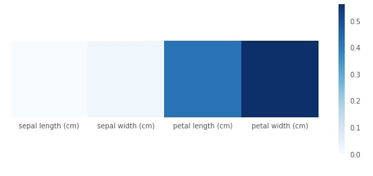
Plotting Feature Importance
We can access the feature importance of each feature in the decision tree through feature_importances_ attributes. We have plotted it as well for better understanding.
print("Feature Importance : %s"%str(grid.best_estimator_.feature_importances_))
with plt.style.context(('seaborn', 'ggplot')):
    plt.figure(figsize=(10,4))
    plt.imshow(grid.best_estimator_.feature_importances_.reshape(1,-1), cmap=plt.cm.Blues, interpolation='nearest')
    plt.xticks(range(4), iris.feature_names)
    plt.yticks([])
    plt.grid(None)
    plt.colorbar();
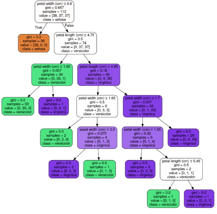
Visualizing Decision Tree Using GraphViz & PyDotPlus
We can visualize the decision tree by using graphviz. Scikit-learn provides export_graphviz() function which can let us convert tree trained to graphviz format. We can then generate a graph from it using the pydotplus library using its method graph_from_dot_data.
We can easily ask questions about flower type based on flower features and get an answer from the decision tree based on True or False answer to the question.
from sklearn.externals.six import StringIO
from sklearn.tree import export_graphviz
from IPython.display import Image
import pydotplus

dot_data = StringIO()

export_graphviz(grid.best_estimator_, out_file=dot_data,
                filled=True, rounded=True,
                special_characters=True,
                class_names=iris.target_names,
                feature_names=iris.feature_names)

graph = pydotplus.graph_from_dot_data(dot_data.getvalue())

Image(graph.create_png())
ExtraTreeClassifier 
ExtraTreeClassifier is commonly referred to as an extremely randomized decision tree. When deciding to split samples into 2 groups based on a feature, random splits are drawn for each of randomly selected features and the best of them is selected.
Fitting Model To Train Data
from sklearn.tree import ExtraTreeClassifier

extra_tree_classifier = ExtraTreeClassifier(random_state=1)
extra_tree_classifier.fit(X_train, Y_train)
Evaluating Trained Model On Test Data.
Almost all models in Scikit-Learn API provides predict() method which can be used to predict target variable on Test Set passed to it.
Y_preds = extra_tree_classifier.predict(X_test)

print(Y_preds)
print(Y_test)

print('Test Accuracy : %.3f'%(Y_preds == Y_test).mean() )
print('Test Accuracy : %.3f'%extra_tree_classifier.score(X_test, Y_test)) ## Score method also evaluates accuracy for classification models.
print('Training Accuracy : %.3f'%extra_tree_classifier.score(X_train, Y_train))
extra_tree_classifier.predict_proba(X_test)[:10]
Finetuning Model By Doing Grid Search On Various Hyperparameters.
ExtraTreeClassifier has same hyperparameters as that of DecisionTreeClassifier
n_features = X.shape[1]
n_samples = X.shape[0]

grid = GridSearchCV(ExtraTreeClassifier(random_state=1), cv=3, n_jobs=-1, verbose=5,
                    param_grid ={
                    'criterion': ['gini', 'entropy'],
                    'max_depth': [None,1,2,3,4,5,6,7],
                    'max_features': [None, 'sqrt', 'auto', 'log2', 0.3,0.5,0.7, n_features//2, n_features//3, ],
                    'min_samples_split': [2,0.3,0.5, n_samples//2, n_samples//3, n_samples//5],
                    'min_samples_leaf':[1, 0.3,0.5, n_samples//2, n_samples//3, n_samples//5]},
                    )

grid.fit(X_train, Y_train)

print('Train Accuracy : %.3f'%grid.best_estimator_.score(X_train, Y_train))
print('Test Accuracy : %.3f'%grid.best_estimator_.score(X_test, Y_test))
print('Best Score Through Grid Search : %.3f'%grid.best_score_)
print('Best Parameters : ',grid.best_params_)
Printing First Few Cross Validation Results
cross_val_results = pd.DataFrame(grid.cv_results_)
print('Number of Various Combinations of Parameters Tried : %d'%len(cross_val_results))

cross_val_results.head() ## Printing first few results.
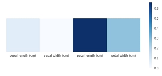
Plotting Feature Importance
print("Feature Importance : %s"%str(grid.best_estimator_.feature_importances_))
with plt.style.context(('seaborn', 'ggplot')):
    plt.figure(figsize=(10,4))
    plt.imshow(grid.best_estimator_.feature_importances_.reshape(1,-1), cmap=plt.cm.Blues, interpolation='nearest')
    plt.xticks(range(4), iris.feature_names)
    plt.yticks([])
    plt.grid(None)
    plt.colorbar();
Please make a note that even though decision trees provides a way to measure target in nonparametric way, it sometimes over-fits data and sometimes under-fits data. hence decision trees are not efficient for dataset with more features and less samples to properly set tree rules/conditions.
DecisionTreeRegressor 
We'll now try loading the Boston dataset provided by sklearn and will try DecisionTreeRegressor on it as well with different depth of the decision tree. We'll also visualize results letter comparing performance on train and test sets with different tree depths.
Loading Data
Below we are loading the IRIS dataset which comes as default with the sklearn package. it returns Bunch object which is almost the same as the dictionary.
boston = datasets.load_boston()
X, Y  = boston.data, boston.target

print('Dataset features names : '+str(boston.feature_names))
print('Dataset features size : '+str(boston.data.shape))
print('Dataset target size : '+str(boston.target.shape))
Splitting Dataset into Train & Test sets
Below we are splitting the Boston dataset into the train set(80%) and test set(20%). We are also using seed(random_state=123) so that we always get the same split and can reproduce results in the future as well.
X_train, X_test,Y_train, Y_test = train_test_split(X, Y, train_size=0.75, test_size=0.25, random_state=1)
print('Train/Test Set Sizes : ', X_train.shape, Y_train.shape, X_test.shape, Y_test.shape)
Fitting Model To Train Data
from sklearn.tree import DecisionTreeRegressor

tree_regressor = DecisionTreeRegressor(random_state=1)
tree_regressor.fit(X_train, Y_train)
Evaluating Trained Model On Test Data.
Almost all models in Scikit-Learn API provides predict() method which can be used to predict target variable on Test Set passed to it.
Y_preds = tree_regressor.predict(X_test)

print(Y_preds[:10])
print(Y_test[:10])

print('Training Coefficient of R^2 : %.3f'%tree_regressor.score(X_train, Y_train))
print('Test Coefficient of R^2 : %.3f'%tree_regressor.score(X_test, Y_test))
Finetuning Model By Doing Grid Search On Various Hyperparameters.
DecisionTreeRegressor has same hyperparameters as DecisionTreeClassifier.
We'll below try various values for the above-mentioned hyperparameters to find the best estimator for our dataset by splitting data into 3-fold cross-validation.
n_features = X.shape[1]
n_samples = X.shape[0]

grid = GridSearchCV(DecisionTreeRegressor(random_state=1), cv=3, n_jobs=-1, verbose=5,
                    param_grid ={
                    'max_depth': [None,1,2,3,4,5,6,7],
                    'max_features': [None, 'sqrt', 'auto', 'log2', 0.3,0.5,0.7, n_features//2, n_features//3, ],
                    'min_samples_split': [2,0.3,0.5, n_samples//2, n_samples//3, n_samples//5],
                    'min_samples_leaf':[1, 0.3,0.5, n_samples//2, n_samples//3, n_samples//5]},
                    )

grid.fit(X_train, Y_train)
print('Train R^2 Score : %.3f'%grid.best_estimator_.score(X_train, Y_train))
print('Test R^2 Score : %.3f'%grid.best_estimator_.score(X_test, Y_test))
print('Best R^2 Score Through Grid Search : %.3f'%grid.best_score_)
print('Best Parameters : ',grid.best_params_)
Printing First Few Cross Validation Results
cross_val_results = pd.DataFrame(grid.cv_results_)
print('Number of Various Combinations of Parameters Tried : %d'%len(cross_val_results))

cross_val_results.head() ## Printing first few results.
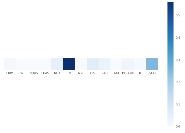
Plotting Feature Importance
print("Feature Importance : %s"%str(grid.best_estimator_.feature_importances_))
with plt.style.context(('seaborn', 'ggplot')):
    plt.figure(figsize=(12,8))
    plt.imshow(grid.best_estimator_.feature_importances_.reshape(1,-1), cmap=plt.cm.Blues, interpolation='nearest')
    plt.xticks(range(13), boston.feature_names)
    plt.yticks([])
    plt.grid(None)
    plt.colorbar();
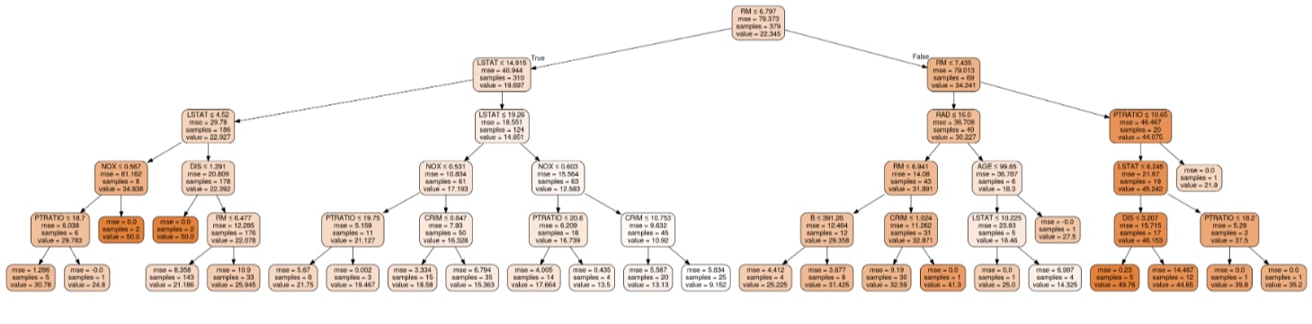
Visualizing Decision Tree Using GraphViz & PyDotPlus
dot_data = StringIO()
export_graphviz(grid.best_estimator_, out_file=dot_data,
                filled=True, rounded=True,
                special_characters=True,
                feature_names=boston.feature_names,)
graph = pydotplus.graph_from_dot_data(dot_data.getvalue())
Image(graph.create_png())
ExtraTreeRegressor 
ExtraTreeRegressor like ExtraTreeClassifier is an extremely randomized decision tree for regression problems. We'll follow the same process as previous examples to explain its usage.
Fitting Model To Train Data
from sklearn.tree import ExtraTreeRegressor

extra_tree_regressor = ExtraTreeRegressor(random_state=1)
extra_tree_regressor.fit(X_train, Y_train)
Evaluating Trained Model On Test Data.
Almost all models in Scikit-Learn API provides predict() method which can be used to predict target variable on Test Set passed to it.
Y_preds = extra_tree_regressor.predict(X_test)

print(Y_preds[:10])
print(Y_test[:10])

print('Training Coefficient of R^2 : %.3f'%extra_tree_regressor.score(X_train, Y_train))
print('Test Coefficient of R^2 : %.3f'%extra_tree_regressor.score(X_test, Y_test))
Finetuning Model By Doing Grid Search On Various Hyperparameters.
ExtraTreeRegressor has same hyperparameters as ExtraTreeClassifier.
We'll below try various values for the above-mentioned hyperparameters to find the best estimator for our dataset by splitting data into 3-fold cross-validation.
n_features = X.shape[1]
n_samples = X.shape[0]

grid = GridSearchCV(ExtraTreeRegressor(random_state=1), cv=3, n_jobs=-1, verbose=5,
                    param_grid ={
                    'max_depth': [None,1,2,3,4,5,6,7],
                    'max_features': [None, 'sqrt', 'auto', 'log2', 0.3,0.5,0.7, n_features//2, n_features//3, ],
                    'min_samples_split': [2,0.3,0.5, n_samples//2, n_samples//3, n_samples//5],
                    'min_samples_leaf':[1, 0.3,0.5, n_samples//2, n_samples//3, n_samples//5]},
                    )

grid.fit(X_train, Y_train)
print('Train R^2 Score : %.3f'%grid.best_estimator_.score(X_train, Y_train))
print('Test R^2 Score : %.3f'%grid.best_estimator_.score(X_test, Y_test))
print('Best R^2 Score Through Grid Search : %.3f'%grid.best_score_)
print('Best Parameters : ',grid.best_params_)
Printing First Few Cross Validation Results
cross_val_results = pd.DataFrame(grid.cv_results_)
print('Number of Various Combinations of Parameters Tried : %d'%len(cross_val_results))

cross_val_results.head() ## Printing first few results.
Plotting Feature Importance
print("Feature Importance : %s"%str(grid.best_estimator_.feature_importances_))
with plt.style.context(('seaborn', 'ggplot')):
    plt.figure(figsize=(12,8))
    plt.imshow(grid.best_estimator_.feature_importances_.reshape(1,-1), cmap=plt.cm.Blues, interpolation='nearest')
    plt.xticks(range(13), boston.feature_names)
    plt.yticks([])
    plt.grid(None)
    plt.colorbar();

The single tree generally overfits data and hence in practice, it's a good idea to combine various decision trees to predict results. The two most common ways to combine multiple decision trees are random forests and gradient boosted trees.
References 
 Sunny Solanki
Sunny Solanki
Intro: Software Developer | Youtuber | Bonsai Enthusiast
About: Sunny Solanki holds a bachelor's degree in Information Technology (2006-2010) from L.D. College of Engineering. Post completion of his graduation, he has 8.5+ years of experience (2011-2019) in the IT Industry (TCS). His IT experience involves working on Python & Java Projects with US/Canada banking clients. Since 2020, he’s primarily concentrating on growing CoderzColumn.
His main areas of interest are AI, Machine Learning, Data Visualization, and Concurrent Programming. He has good hands-on with Python and its ecosystem libraries.
Apart from his tech life, he prefers reading biographies and autobiographies. And yes, he spends his leisure time taking care of his plants and a few pre-Bonsai trees.
Contact: sunny.2309@yahoo.in


![YouTube Subscribe]() Comfortable Learning through Video Tutorials?
Comfortable Learning through Video Tutorials?
If you are more comfortable learning through video tutorials then we would recommend that you subscribe to our YouTube channel.
![Need Help]() Stuck Somewhere? Need Help with Coding? Have Doubts About the Topic/Code?
Stuck Somewhere? Need Help with Coding? Have Doubts About the Topic/Code?
 Stuck Somewhere? Need Help with Coding? Have Doubts About the Topic/Code?
When going through coding examples, it's quite common to have doubts and errors.
If you have doubts about some code examples or are stuck somewhere when trying our code, send us an email at coderzcolumn07@gmail.com. We'll help you or point you in the direction where you can find a solution to your problem.
You can even send us a mail if you are trying something new and need guidance regarding coding. We'll try to respond as soon as possible.
![Share Views]() Want to Share Your Views? Have Any Suggestions?
Want to Share Your Views? Have Any Suggestions?
 Want to Share Your Views? Have Any Suggestions?
If you want to
- provide some suggestions on topic
- share your views
- include some details in tutorial
- suggest some new topics on which we should create tutorials/blogs
 sklearn, decision-trees