Updated On : Nov-15,2020 Time Investment : ~20 mins

Pyinstrument - Statistical Profiler for Python Code

Pyinstrument is a statistical python profiler which records call stack every 1 ms rather than recording the whole trace. This is done in order to avoid profiling overhead which can increase a lot if some functions are getting called many times and not taking that much time to complete. This kind of behavior can even distort results by highlighting part of the code/function which might not be slow but getting called many times completing faster. In a way it kind of tries to avoid profiling noise by removing profiling information of faster parts of code. This kind of behavior also has a drawback that some of the function calls which ran quite fast will not be recorded but they are already fast. Pyinstrument uses an OS feature called signals to ask OS to send a signal and handle signals using a python signal handler (PyEval_SetProfile) for recording every 1 ms. Pyinstrument has other limitations due to its design that it can't profile the multi-threaded code. It'll only be recording the main thread. As Pyinstrument only takes recordings every 1 ms seconds, it runs faster than python profilers like cProfile, profile, etc. Apart from this, Pyinstrument records wall time (not CPU time) which includes all database call wait, network packet wait, file i/o wait, etc. The main reason for measuring wall-clock time given by the author of Pyinstrument is that Python is most commonly used as glue language connecting different services designed in different languages and users are interested in knowing whether slowness is due to Python or some other services. Pyinstrument also gives us a trace of only functions used in our script rather than flooding output with all internal function calls of python and other C function calls. Pyinstrument also lets developer format profiling output in different formats like HTML, JSON, text, or user defined class for rendering output.

As a part of this tutorial, we'll explain with simple examples of how we can use Pyinstrument to profile our python code. We'll explain the usage of profiler in a two way:

  • Profiling script from the command line.
  • Profiling script with Profiler instance in Python code itself.

Profiling script from the command line

As a part of this section, we'll explain how we can profile script from the command line using various options available from Pyinstrument. We'll try to cover all possible options available through various examples.

Example 1: Simply Profiling Script

Our first example involves profiling results generation for a simple python script using Pyinstrument. We have created a simple python script which loops 1000000 times generating two random numbers, adding them to generate a sum, and then adding that sum to the list before returning the list. We have kept this script in a file named pyinstrument_ex1.py in a folder named profiling_examples. We'll be reusing the script in the future examples as well.

CODE

import random

def add(a, b):
    return a+b


def get_sum_of_list():
    final_list = []
    for i in range(1000000):
        rand1 = random.randint(1,100)
        rand2 = random.randint(1,100)
        out = add(rand1, rand2)
        final_list.append(out)
    return final_list


if __name__ == "__main__":
    l = get_sum_of_list()
#    print(l)

Below we have profiled script using Pyinstrument without default options. Please make a note that we are using the ! symbol which lets us execute a shell command from Jupyter Notebook. This command can be run exactly the same way from a shell.

!pyinstrument profiling_examples/pyinstrument_ex1.py
  _     ._   __/__   _ _  _  _ _/_   Recorded: 16:39:21  Samples:  2192
 /_//_/// /_\ / //_// / //_'/ //     Duration: 2.199     CPU time: 2.197
/   _/                      v3.2.0

Program: profiling_examples/pyinstrument_ex1.py

2.199 <module>  pyinstrument_ex1.py:1
└─ 2.199 get_sum_of_list  pyinstrument_ex1.py:7
   ├─ 1.714 randint  random.py:218
   │     [6 frames hidden]  random
   │        1.442 randrange  random.py:174
   │        ├─ 0.734 [self]
   │        └─ 0.708 _randbelow  random.py:224
   │           ├─ 0.501 [self]
   │           ├─ 0.153 Random.getrandbits  ../<built-in>:0
   │           └─ 0.054 int.bit_length  ../<built-in>:0
   ├─ 0.405 [self]
   ├─ 0.050 add  pyinstrument_ex1.py:3
   └─ 0.030 list.append  ../<built-in>:0

To view this report with different options, run:
    pyinstrument --load-prev 2020-11-12T16-39-21 [options]

The output of profiling generated by Pyinstrument is formatted in a tree-like structure. It'll be showing total time at the top and then the time taken by sub-functions will be shown one level down the tree. It also has color-coded time taken by various functions. The [self] in output refers to the time taken by function excluding other functions called in that function. FOr example, if we have taken randrange then two nodes below it are [self] and _randbelow where [self] refers to the time taken by randrange excluding time taken by _randbelow. The same goes for get_sum_of_list function which has four children (randint(), [self], add(), list.append()). It might happen that some of the functions of the script do not get recorded by Pyinstrument because it can be too fast and Pyinstrument takes sampling every 0.001 seconds.

Example 2: Load Previous Profiling Result

Pyinstrument also stores profiling results of the last execution and gives us ID which we can use to reprint the results as well as formating that results in a different formats. Below we have explained how we can reload previous profiling results using the --load-prev option.

!pyinstrument --load-prev 2020-11-12T16-39-21
  _     ._   __/__   _ _  _  _ _/_   Recorded: 16:39:21  Samples:  2192
 /_//_/// /_\ / //_// / //_'/ //     Duration: 2.199     CPU time: 2.197
/   _/                      v3.2.0

Program: profiling_examples/pyinstrument_ex1.py

2.199 <module>  ../../profiling_examples/pyinstrument_ex1.py:1
└─ 2.199 get_sum_of_list  ../../profiling_examples/pyinstrument_ex1.py:7
   ├─ 1.714 randint  random.py:218
   │     [6 frames hidden]  random
   │        1.442 randrange  random.py:174
   │        ├─ 0.734 [self]
   │        └─ 0.708 _randbelow  random.py:224
   │           ├─ 0.501 [self]
   │           ├─ 0.153 Random.getrandbits  ../../<built-in>:0
   │           └─ 0.054 int.bit_length  ../../<built-in>:0
   ├─ 0.405 [self]
   ├─ 0.050 add  ../../profiling_examples/pyinstrument_ex1.py:3
   └─ 0.030 list.append  ../../<built-in>:0

To view this report with different options, run:
    pyinstrument --load-prev 2020-11-12T16-39-21 [options]

Example 3: Saving Profiling to a File

We'll be explaining how we can save the output of profiling to a file as a part of our third example. We have designed a new python script that has three functions which generate an average of 100000 random numbers between 1-100 each taking a different time. We have introduced artificial time in each function so that it looks like each time different time. We are then calling each function and printing their results. We have stored code of script in a file named pyinstrument_ex2.py kept in a folder named profiling_examples. We'll be using the same script in our future examples as well.

CODE

import time
import random

def very_slow_random_generator():
    time.sleep(5)
    arr = [random.randint(1,100) for i in range(100000)]
    return sum(arr) / len(arr)

def slow_random_generator():
    time.sleep(2)
    arr = [random.randint(1,100) for i in range(100000)]
    return sum(arr) / len(arr)

def fast_random_generator():
    time.sleep(1)
    arr = [random.randint(1,100) for i in range(100000)]
    return sum(arr) / len(arr)

def main_func():
    result = fast_random_generator()
    print(result)

    result = slow_random_generator()
    print(result)

    result = very_slow_random_generator()
    print(result)

main_func()

Pyinstrument provides us with an option named -o or --outfile which can let us save profiling output to file.

  • -o FILE_NAME
  • --output==FILE_NAME

Below we have stored profiling results to a file named pyinstrument_ex2_out.out. We are then also displaying file contents.

!pyinstrument -o pyinstrument_ex2_out.out profiling_examples/pyinstrument_ex2.py
50.56541
50.42884
50.53442
To view this report with different options, run:
    pyinstrument --load-prev 2020-11-12T16-50-27 [options]

!cat pyinstrument_ex2_out.out
  _     ._   __/__   _ _  _  _ _/_   Recorded: 16:50:27  Samples:  309
 /_//_/// /_\ / //_// / //_'/ //     Duration: 8.316     CPU time: 0.308
/   _/                      v3.2.0

Program: profiling_examples/pyinstrument_ex2.py

8.316 <module>  pyinstrument_ex2.py:1
└─ 8.316 main_func  pyinstrument_ex2.py:19
   ├─ 5.107 very_slow_random_generator  pyinstrument_ex2.py:4
   │  ├─ 5.005 sleep  ../<built-in>:0
   │  └─ 0.102 <listcomp>  pyinstrument_ex2.py:6
   │     └─ 0.092 randint  random.py:218
   │           [6 frames hidden]  random
   ├─ 2.105 slow_random_generator  pyinstrument_ex2.py:9
   │  ├─ 2.003 sleep  ../<built-in>:0
   │  └─ 0.101 <listcomp>  pyinstrument_ex2.py:11
   │     └─ 0.089 randint  random.py:218
   │           [6 frames hidden]  random
   └─ 1.103 fast_random_generator  pyinstrument_ex2.py:14
      ├─ 1.001 sleep  ../<built-in>:0
      └─ 0.102 <listcomp>  pyinstrument_ex2.py:16
         └─ 0.090 randint  random.py:218
               [6 frames hidden]  random

Example 4: Rending Output in a HTML/JSON Formats

In our fourth example, we'll explain how we can format output in an HTML and JSON format. Pyinstrument lets us format our profiling results using the -r or --renderer option.

  • -r RENDERED
  • --rendered=RENDERER

Below we have formatted output in an HTML format. It'll store results in a temporary file and open it in a new tab in a web browser.

!pyinstrument -r html profiling_examples/pyinstrument_ex2.py
50.4177
50.5274
50.62186
stdout is a terminal, so saved profile output to /tmp/tmpvu1m9t9_.html

Pyinstrument - Statistical Profiler for Python Code

Below we have stored HTML output in a file.

!pyinstrument -r html -o pyinstrument_ex1.html profiling_examples/pyinstrument_ex2.py
50.5085
50.43991
50.58166

Below we have formatted output in a JSON format for our first script from the first example. We have then included code that loads content from file and prints it as well.

!pyinstrument -r json -o pyinstrument_ex1.json profiling_examples/pyinstrument_ex1.py
import json

trace = json.load(open("pyinstrument_ex1.json"))
print(json.dumps(trace, indent=2))
{
  "start_time": 1605180221.199558,
  "duration": 2.288824,
  "sample_count": 2286,
  "program": "profiling_examples/pyinstrument_ex1.py",
  "cpu_time": 2.288463,
  "root_frame": {
    "function": "<module>",
    "file_path_short": "pyinstrument_ex1.py",
    "file_path": "profiling_examples/pyinstrument_ex1.py",
    "line_no": 1,
    "time": 2.288728,
    "is_application_code": true,
    "children": [
      {
        "function": "get_sum_of_list",
        "file_path_short": "pyinstrument_ex1.py",
        "file_path": "profiling_examples/pyinstrument_ex1.py",
        "line_no": 7,
        "time": 2.288728,
        "is_application_code": true,
        "children": [
          {
            "function": "randint",
            "file_path_short": "random.py",
            "file_path": "/home/sunny/anaconda3/lib/python3.7/random.py",
            "line_no": 218,
            "time": 1.799895,
            "is_application_code": false,
            "children": [
              {
                "function": "randrange",
                "file_path_short": "random.py",
                "file_path": "/home/sunny/anaconda3/lib/python3.7/random.py",
                "line_no": 174,
                "time": 1.493957,
                "is_application_code": false,
                "children": [
                  {
                    "function": "_randbelow",
                    "file_path_short": "random.py",
                    "file_path": "/home/sunny/anaconda3/lib/python3.7/random.py",
                    "line_no": 224,
                    "time": 0.794717,
                    "is_application_code": false,
                    "children": [
                      {
                        "function": "[self]",
                        "file_path_short": "",
                        "file_path": "/home/sunny/anaconda3/lib/python3.7/random.py",
                        "line_no": 224,
                        "time": 0.530674,
                        "is_application_code": false,
                        "children": [],
                        "group_id": "6ba322a8-2ada-4c5d-ba0b-69d35ec2572f"
                      },
                      {
                        "function": "Random.getrandbits",
                        "file_path_short": "../<built-in>",
                        "file_path": "<built-in>",
                        "line_no": 0,
                        "time": 0.179017,
                        "is_application_code": false,
                        "children": []
                      },
                      {
                        "function": "int.bit_length",
                        "file_path_short": "../<built-in>",
                        "file_path": "<built-in>",
                        "line_no": 0,
                        "time": 0.085026,
                        "is_application_code": false,
                        "children": []
                      }
                    ],
                    "group_id": "6ba322a8-2ada-4c5d-ba0b-69d35ec2572f"
                  },
                  {
                    "function": "[self]",
                    "file_path_short": "",
                    "file_path": "/home/sunny/anaconda3/lib/python3.7/random.py",
                    "line_no": 174,
                    "time": 0.69924,
                    "is_application_code": false,
                    "children": [],
                    "group_id": "6ba322a8-2ada-4c5d-ba0b-69d35ec2572f"
                  }
                ],
                "group_id": "6ba322a8-2ada-4c5d-ba0b-69d35ec2572f"
              },
              {
                "function": "[self]",
                "file_path_short": "",
                "file_path": "/home/sunny/anaconda3/lib/python3.7/random.py",
                "line_no": 218,
                "time": 0.305937,
                "is_application_code": false,
                "children": [],
                "group_id": "6ba322a8-2ada-4c5d-ba0b-69d35ec2572f"
              }
            ],
            "group_id": "6ba322a8-2ada-4c5d-ba0b-69d35ec2572f"
          },
          {
            "function": "[self]",
            "file_path_short": "",
            "file_path": "profiling_examples/pyinstrument_ex1.py",
            "line_no": 7,
            "time": 0.409855,
            "is_application_code": false,
            "children": []
          },
          {
            "function": "add",
            "file_path_short": "pyinstrument_ex1.py",
            "file_path": "profiling_examples/pyinstrument_ex1.py",
            "line_no": 3,
            "time": 0.052972,
            "is_application_code": true,
            "children": []
          },
          {
            "function": "list.append",
            "file_path_short": "../<built-in>",
            "file_path": "<built-in>",
            "line_no": 0,
            "time": 0.026007,
            "is_application_code": false,
            "children": []
          }
        ]
      }
    ]
  }
}

Pyinstrument also provides an option named --no-color which lets us instruct Pyinstrument to not use color coding when printing profiling results.

!pyinstrument --no-color profiling_examples/pyinstrument_ex2.py
50.52441
50.60048
50.58576

  _     ._   __/__   _ _  _  _ _/_   Recorded: 16:51:40  Samples:  333
 /_//_/// /_\ / //_// / //_'/ //     Duration: 8.340     CPU time: 0.332
/   _/                      v3.2.0

Program: profiling_examples/pyinstrument_ex2.py

8.340 <module>  pyinstrument_ex2.py:1
└─ 8.340 main_func  pyinstrument_ex2.py:19
   ├─ 5.128 very_slow_random_generator  pyinstrument_ex2.py:4
   │  ├─ 5.005 sleep  ../<built-in>:0
   │  └─ 0.121 <listcomp>  pyinstrument_ex2.py:6
   │     └─ 0.104 randint  random.py:218
   │           [6 frames hidden]  random
   ├─ 2.107 slow_random_generator  pyinstrument_ex2.py:9
   │  ├─ 2.003 sleep  ../<built-in>:0
   │  └─ 0.103 <listcomp>  pyinstrument_ex2.py:11
   │     └─ 0.085 randint  random.py:218
   │           [6 frames hidden]  random
   └─ 1.105 fast_random_generator  pyinstrument_ex2.py:14
      ├─ 1.001 sleep  ../<built-in>:0
      └─ 0.104 <listcomp>  pyinstrument_ex2.py:16
         └─ 0.094 randint  random.py:218
               [6 frames hidden]  random

To view this report with different options, run:
    pyinstrument --load-prev 2020-11-12T16-51-40 [options]

Example 5: Render Output as a Timeline in Exact Execution Order

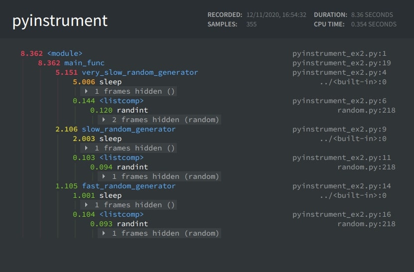
Pyinstrument provides us with an option named -t or --timeline which will order profiling results in an order in which they are executed. If we don't use these options then profiling results will be ordered by the time taken by functions. We can notice from the output of this execution that it first shows fast_random_generator then slow_random_generator and at last very_slow_random_generator whereas this order was reverse in all previous profiling results.

!pyinstrument -t profiling_examples/pyinstrument_ex2.py
50.45461
50.56285
50.44026

  _     ._   __/__   _ _  _  _ _/_   Recorded: 17:01:19  Samples:  308
 /_//_/// /_\ / //_// / //_'/ //     Duration: 8.315     CPU time: 0.307
/   _/                      v3.2.0

Program: profiling_examples/pyinstrument_ex2.py

8.315 <module>  pyinstrument_ex2.py:1
└─ 8.315 main_func  pyinstrument_ex2.py:19
   ├─ 1.102 fast_random_generator  pyinstrument_ex2.py:14
   │  ├─ 1.001 sleep  ../<built-in>:0
   │  └─ 0.101 <listcomp>  pyinstrument_ex2.py:16
   ├─ 2.104 slow_random_generator  pyinstrument_ex2.py:9
   │  ├─ 2.003 sleep  ../<built-in>:0
   │  └─ 0.101 <listcomp>  pyinstrument_ex2.py:11
   └─ 5.109 very_slow_random_generator  pyinstrument_ex2.py:4
      ├─ 5.006 sleep  ../<built-in>:0
      └─ 0.102 <listcomp>  pyinstrument_ex2.py:6

To view this report with different options, run:
    pyinstrument --load-prev 2020-11-12T17-01-19 [options]

Example 6: Show All Traces Including Default Libraries

We can inform Pyinstrument to show us profiling results of all default libraries used in a code by using the --show-all option. Below we have first compiled code normally and then used the --show-all option in the next cell to show default library cells.

!pyinstrument -t profiling_examples/pyinstrument_ex2.py
50.48434
50.51676
50.4761

  _     ._   __/__   _ _  _  _ _/_   Recorded: 17:05:28  Samples:  309
 /_//_/// /_\ / //_// / //_'/ //     Duration: 8.315     CPU time: 0.306
/   _/                      v3.2.0

Program: profiling_examples/pyinstrument_ex2.py

8.315 <module>  pyinstrument_ex2.py:1
└─ 8.315 main_func  pyinstrument_ex2.py:19
   ├─ 1.103 fast_random_generator  pyinstrument_ex2.py:14
   │  ├─ 1.001 sleep  ../<built-in>:0
   │  └─ 0.101 <listcomp>  pyinstrument_ex2.py:16
   ├─ 2.106 slow_random_generator  pyinstrument_ex2.py:9
   │  ├─ 2.002 sleep  ../<built-in>:0
   │  └─ 0.102 <listcomp>  pyinstrument_ex2.py:11
   └─ 5.106 very_slow_random_generator  pyinstrument_ex2.py:4
      ├─ 5.005 sleep  ../<built-in>:0
      └─ 0.100 <listcomp>  pyinstrument_ex2.py:6

To view this report with different options, run:
    pyinstrument --load-prev 2020-11-12T17-05-28 [options]

 !pyinstrument --load-prev 2020-11-12T17-05-28 --show-all
  _     ._   __/__   _ _  _  _ _/_   Recorded: 17:05:28  Samples:  309
 /_//_/// /_\ / //_// / //_'/ //     Duration: 8.315     CPU time: 0.306
/   _/                      v3.2.0

Program: profiling_examples/pyinstrument_ex2.py

8.315 <module>  ../../profiling_examples/pyinstrument_ex2.py:1
└─ 8.315 main_func  ../../profiling_examples/pyinstrument_ex2.py:19
   ├─ 5.106 very_slow_random_generator  ../../profiling_examples/pyinstrument_ex2.py:4
   │  ├─ 5.005 sleep  ../../<built-in>:0
   │  └─ 0.100 <listcomp>  ../../profiling_examples/pyinstrument_ex2.py:6
   │     └─ 0.089 randint  random.py:218
   │           [6 frames hidden]  random
   ├─ 2.106 slow_random_generator  ../../profiling_examples/pyinstrument_ex2.py:9
   │  ├─ 2.002 sleep  ../../<built-in>:0
   │  └─ 0.102 <listcomp>  ../../profiling_examples/pyinstrument_ex2.py:11
   │     └─ 0.089 randint  random.py:218
   │           [6 frames hidden]  random
   └─ 1.103 fast_random_generator  ../../profiling_examples/pyinstrument_ex2.py:14
      ├─ 1.001 sleep  ../../<built-in>:0
      └─ 0.101 <listcomp>  ../../profiling_examples/pyinstrument_ex2.py:16
         └─ 0.091 randint  random.py:218
               [6 frames hidden]  random

To view this report with different options, run:
    pyinstrument --load-prev 2020-11-12T17-05-28 [options]

Example 7: Hide Unwanted File Traces

Pyinstrument lets us hide files for which we don't want to include profiling results by using --hide=EXPR and --hide-regex=REGEX options.

  • --hide=EXPR - Here EXPR is a glob path matching expression commonly used in UNIX shell.
  • --hide-regex=REGEX - Here REGEX is a regular expression which will match paths.

Below we have first normally profiled our pyinstrument_ex2.py script. We have then removed the hidden frame from profiling output using options.

!pyinstrument profiling_examples/pyinstrument_ex2.py
50.54397
50.67017
50.62488

  _     ._   __/__   _ _  _  _ _/_   Recorded: 17:12:13  Samples:  310
 /_//_/// /_\ / //_// / //_'/ //     Duration: 8.317     CPU time: 0.309
/   _/                      v3.2.0

Program: profiling_examples/pyinstrument_ex2.py

8.317 <module>  pyinstrument_ex2.py:1
└─ 8.317 main_func  pyinstrument_ex2.py:19
   ├─ 5.108 very_slow_random_generator  pyinstrument_ex2.py:4
   │  ├─ 5.005 sleep  ../<built-in>:0
   │  └─ 0.102 <listcomp>  pyinstrument_ex2.py:6
   │     └─ 0.090 randint  random.py:218
   │           [6 frames hidden]  random
   ├─ 2.105 slow_random_generator  pyinstrument_ex2.py:9
   │  ├─ 2.003 sleep  ../<built-in>:0
   │  └─ 0.101 <listcomp>  pyinstrument_ex2.py:11
   │     └─ 0.091 randint  random.py:218
   │           [6 frames hidden]  random
   └─ 1.103 fast_random_generator  pyinstrument_ex2.py:14
      ├─ 1.001 sleep  ../<built-in>:0
      └─ 0.102 <listcomp>  pyinstrument_ex2.py:16
         └─ 0.094 randint  random.py:218
               [6 frames hidden]  random

To view this report with different options, run:
    pyinstrument --load-prev 2020-11-12T17-12-13 [options]

!pyinstrument --load-prev 2020-11-12T17-12-13 --hide="*/random/*"
  _     ._   __/__   _ _  _  _ _/_   Recorded: 17:12:13  Samples:  310
 /_//_/// /_\ / //_// / //_'/ //     Duration: 8.317     CPU time: 0.309
/   _/                      v3.2.0

Program: profiling_examples/pyinstrument_ex2.py

8.317 <module>  ../../profiling_examples/pyinstrument_ex2.py:1
└─ 8.317 main_func  ../../profiling_examples/pyinstrument_ex2.py:19
   ├─ 5.108 very_slow_random_generator  ../../profiling_examples/pyinstrument_ex2.py:4
   │  ├─ 5.005 sleep  ../../<built-in>:0
   │  └─ 0.102 <listcomp>  ../../profiling_examples/pyinstrument_ex2.py:6
   │     └─ 0.090 randint  random.py:218
   ├─ 2.105 slow_random_generator  ../../profiling_examples/pyinstrument_ex2.py:9
   │  ├─ 2.003 sleep  ../../<built-in>:0
   │  └─ 0.101 <listcomp>  ../../profiling_examples/pyinstrument_ex2.py:11
   │     └─ 0.091 randint  random.py:218
   └─ 1.103 fast_random_generator  ../../profiling_examples/pyinstrument_ex2.py:14
      ├─ 1.001 sleep  ../../<built-in>:0
      └─ 0.102 <listcomp>  ../../profiling_examples/pyinstrument_ex2.py:16
         └─ 0.094 randint  random.py:218

To view this report with different options, run:
    pyinstrument --load-prev 2020-11-12T17-12-13 [options]

!pyinstrument --load-prev 2020-11-12T17-12-13 --hide-regex="random"
  _     ._   __/__   _ _  _  _ _/_   Recorded: 17:12:13  Samples:  310
 /_//_/// /_\ / //_// / //_'/ //     Duration: 8.317     CPU time: 0.309
/   _/                      v3.2.0

Program: profiling_examples/pyinstrument_ex2.py

8.317 <module>  ../../profiling_examples/pyinstrument_ex2.py:1
└─ 8.317 main_func  ../../profiling_examples/pyinstrument_ex2.py:19
   ├─ 5.108 very_slow_random_generator  ../../profiling_examples/pyinstrument_ex2.py:4
   │  ├─ 5.005 sleep  ../../<built-in>:0
   │  └─ 0.102 <listcomp>  ../../profiling_examples/pyinstrument_ex2.py:6
   │     └─ 0.090 randint  random.py:218
   ├─ 2.105 slow_random_generator  ../../profiling_examples/pyinstrument_ex2.py:9
   │  ├─ 2.003 sleep  ../../<built-in>:0
   │  └─ 0.101 <listcomp>  ../../profiling_examples/pyinstrument_ex2.py:11
   │     └─ 0.091 randint  random.py:218
   └─ 1.103 fast_random_generator  ../../profiling_examples/pyinstrument_ex2.py:14
      ├─ 1.001 sleep  ../../<built-in>:0
      └─ 0.102 <listcomp>  ../../profiling_examples/pyinstrument_ex2.py:16
         └─ 0.094 randint  random.py:218

To view this report with different options, run:
    pyinstrument --load-prev 2020-11-12T17-12-13 [options]

It sometimes happens that --hide or --hide-regex is removing all files matching that pattern and we want to include some of the files then we can override it using the below-mentioned option. These options will again show that file results.

  • --show=EXPR
  • --show-regex=REGEX

Example 8: Profile a Module

Pyinstrument can be used to profile a python module as well using the -m option. Below we have a profiled random module.

!pyinstrument -m random
2000 times random
0.001 sec, avg 0.496516, stddev 0.289375, min 0.000323447, max 0.999378

2000 times normalvariate
0.002 sec, avg -0.0217509, stddev 0.985416, min -3.13354, max 3.32162

2000 times lognormvariate
0.003 sec, avg 1.61296, stddev 1.93294, min 0.0318588, max 21.6617

2000 times vonmisesvariate
0.003 sec, avg 3.16923, stddev 2.28078, min 0.000185524, max 6.27983

2000 times gammavariate
0.002 sec, avg 0.0102363, stddev 0.0895552, min 1.49066e-291, max 2.17814

2000 times gammavariate
0.002 sec, avg 0.101093, stddev 0.314004, min 5.14684e-36, max 3.38571

2000 times gammavariate
0.002 sec, avg 0.204238, stddev 0.644938, min 1.48283e-52, max 14.0109

2000 times gammavariate
0.002 sec, avg 0.527816, stddev 0.760323, min 4.3402e-07, max 7.02732

2000 times gammavariate
0.002 sec, avg 0.885683, stddev 0.942166, min 7.60176e-05, max 8.18968

2000 times gammavariate
0.002 sec, avg 1.03951, stddev 1.02211, min 0.000945075, max 7.5032

2000 times gammavariate
0.003 sec, avg 1.96332, stddev 1.3751, min 0.0432269, max 11.644

2000 times gammavariate
0.003 sec, avg 20.051, stddev 4.4533, min 8.54435, max 38.4094

2000 times gammavariate
0.003 sec, avg 200.149, stddev 13.915, min 155.413, max 253.811

2000 times gauss
0.002 sec, avg -0.0149898, stddev 1.02317, min -3.793, max 3.26005

2000 times betavariate
0.005 sec, avg 0.502823, stddev 0.190558, min 0.0399309, max 0.970535

2000 times triangular
0.002 sec, avg 0.447954, stddev 0.20453, min 0.0275026, max 0.991511


  _     ._   __/__   _ _  _  _ _/_   Recorded: 17:15:22  Samples:  38
 /_//_/// /_\ / //_// / //_'/ //     Duration: 0.039     CPU time: 0.039
/   _/                      v3.2.0

Program: random

0.038 <module>  ../../<string>:1
└─ 0.038 run_module  runpy.py:195
      [22 frames hidden]  runpy, random
         0.038 _test_generator  random.py:702
         ├─ 0.013 gammavariate  random.py:504
         │  ├─ 0.009 [self]
         │  ├─ 0.002 Random.random  ../../<built-in>:0
         │  ├─ 0.001 sqrt  ../../<built-in>:0
         │  └─ 0.001 exp  ../../<built-in>:0
         │  0.006 gammavariate  random.py:504
         │  └─ 0.001 log  ../../<built-in>:0
         ├─ 0.004 min  ../../<built-in>:0
         ├─ 0.002 max  ../../<built-in>:0
         ├─ 0.002 vonmisesvariate  random.py:456
         │  ├─ 0.001 acos  ../../<built-in>:0
         ├─ 0.002 gauss  random.py:576
         │  ├─ 0.001 Random.random  ../../<built-in>:0
         │  0.001 normalvariate  random.py:400
         │  └─ 0.001 log  ../../<built-in>:0

To view this report with different options, run:
    pyinstrument --load-prev 2020-11-12T17-15-22 [options]

Profiling script with Profiler instance in Python code itself.

As a part of this section, we'll explain with a few examples of how we can use the Profile instance to monitor a particular part of the code if we don't want to monitor the total code.

Example 1: Simple Profiling With Profile Instance

Our first example demonstrates how we can profile a python code using the Profile instance. We first need to create an instance of Profile. We then need to cover part of the code which we want to profile between start() and stop() methods of profile instance. Below we have again produced the same code that we had used in the previous section. We have covered part where we are calling get_sum_of_list() method between start() and stop() methods.

import pyinstrument
import random

profiler = pyinstrument.Profiler(interval=0.01) ## Profiler

def add(a, b):
    return a+b


def get_sum_of_list():
    final_list = []
    for i in range(1000000):
        rand1 = random.randint(1,100)
        rand2 = random.randint(1,100)
        out = add(rand1, rand2)
        final_list.append(out)
    return final_list

profiler.start() ## Start Profiling

l = get_sum_of_list()

profiler.stop(); ## Stop Profiling

output_text()

The profiler instance has a method named output_text() which can let us print results in a text format. It has options to show Unicode text, colored text, show all profiled frames, and time lined output. We have first printed uncolored text output followed by colored text output.

print(profiler.output_text(unicode=False, color=False, show_all=False, timeline=False))
  _     ._   __/__   _ _  _  _ _/_   Recorded: 17:39:18  Samples:  224
 /_//_/// /_\ / //_// / //_'/ //     Duration: 2.242     CPU time: 2.242
/   _/                      v3.2.0

Program: /home/sunny/anaconda3/lib/python3.7/site-packages/ipykernel_launcher.py -f /home/sunny/.local/share/jupyter/runtime/kernel-c450ef03-3d9f-4980-8dc2-314d5fcbe1ae.json

2.240 run_code  IPython/core/interactiveshell.py:3287
`- 2.240 <module>  <ipython-input-112-0ae0de433d77>:21
   `- 2.240 get_sum_of_list  <ipython-input-112-0ae0de433d77>:10
      |- 1.711 randint  random.py:218
      |     [10 frames hidden]  random, <built-in>
      |        1.390 randrange  random.py:174
      |        |- 0.770 _randbelow  random.py:224
      |        |  |- 0.510 [self]
      |        `- 0.620 [self]
      |- 0.440 [self]
      |- 0.050 list.append  <built-in>:0
      |     [2 frames hidden]  <built-in>
      `- 0.040 add  <ipython-input-112-0ae0de433d77>:6


print(profiler.output_text(color=True))
  _     ._   __/__   _ _  _  _ _/_   Recorded: 17:39:18  Samples:  224
 /_//_/// /_\ / //_// / //_'/ //     Duration: 2.242     CPU time: 2.242
/   _/                      v3.2.0

Program: /home/sunny/anaconda3/lib/python3.7/site-packages/ipykernel_launcher.py -f /home/sunny/.local/share/jupyter/runtime/kernel-c450ef03-3d9f-4980-8dc2-314d5fcbe1ae.json

2.240 run_code  IPython/core/interactiveshell.py:3287
`- 2.240 <module>  <ipython-input-112-0ae0de433d77>:21
   `- 2.240 get_sum_of_list  <ipython-input-112-0ae0de433d77>:10
      |- 1.711 randint  random.py:218
      |     [10 frames hidden]  random, <built-in>
      |        1.390 randrange  random.py:174
      |        |- 0.770 _randbelow  random.py:224
      |        |  |- 0.510 [self]
      |        `- 0.620 [self]
      |- 0.440 [self]
      |- 0.050 list.append  <built-in>:0
      |     [2 frames hidden]  <built-in>
      `- 0.040 add  <ipython-input-112-0ae0de433d77>:6


Example 2: Rendering Output In HTML/JSON Format

We'll be explaining how we can format output in HTML and JSON format as a part of this example. We have reproduced code that we had used in the previous section. We have also created a profiler instance and then covered code where we are calling the main function between start() and stop() methods for profiling.

import pyinstrument
import time
import random

def very_slow_random_generator():
    time.sleep(5)
    arr = [random.randint(1,100) for i in range(100000)]
    return sum(arr) / len(arr)

def slow_random_generator():
    time.sleep(2)
    arr = [random.randint(1,100) for i in range(100000)]
    return sum(arr) / len(arr)

def fast_random_generator():
    time.sleep(1)
    arr = [random.randint(1,100) for i in range(100000)]
    return sum(arr) / len(arr)

def main_func():
    result = fast_random_generator()
    print(result)

    result = slow_random_generator()
    print(result)

    result = very_slow_random_generator()
    print(result)


profiler = pyinstrument.Profiler(interval=0.01) ## Profiler

profiler.start()

main_func()

profiler.stop();
50.50344
50.6106
50.5112

output_html()

The profiler instance has a method named output_html() which will generate output as HTML string. We have stored output to a file named pyinstrument_ex2_2.html file.

output = profiler.output_html()

fp = open("pyinstrument_ex2_2.html", "w")
fp.write(output)
fp.close();

Pyinstrument - Statistical Profiler for Python Code

open_in_browser()

The open_in_browser() method saves HTML output to a temporary file and then opens it in a new tab in the web browser.

profiler.open_in_browser()
'/tmp/tmppqss45i0.html'

Pyinstrument - Statistical Profiler for Python Code

output()

The output() method lets us format output in an HTML or JSON format by using a different renderers. Below we have generated JSON formatted output and saved it to a file. We have then reloaded JSON formatted output and printed it to standard output.

from pyinstrument.renderers import JSONRenderer, HTMLRenderer
json_output = profiler.output(JSONRenderer(show_all=False, timeline=False))

fp = open("pyinstrument_ex2.json", "w")
fp.write(json_output)
fp.close();
import json

trace = json.load(open("pyinstrument_ex2.json"))
print(json.dumps(trace, indent=2))
{
  "start_time": 1605182449.741764,
  "duration": 8.322173,
  "sample_count": 33,
  "program": "/home/sunny/anaconda3/lib/python3.7/site-packages/ipykernel_launcher.py -f /home/sunny/.local/share/jupyter/runtime/kernel-c450ef03-3d9f-4980-8dc2-314d5fcbe1ae.json",
  "cpu_time": 0.318794,
  "root_frame": {
    "function": "run_code",
    "file_path_short": "IPython/core/interactiveshell.py",
    "file_path": "/home/sunny/anaconda3/lib/python3.7/site-packages/IPython/core/interactiveshell.py",
    "line_no": 3287,
    "time": 8.318942,
    "is_application_code": false,
    "children": [
      {
        "function": "<module>",
        "file_path_short": "<ipython-input-92-ce52eeb8f0bb>",
        "file_path": "<ipython-input-92-ce52eeb8f0bb>",
        "line_no": 35,
        "time": 8.318942,
        "is_application_code": true,
        "children": [
          {
            "function": "main_func",
            "file_path_short": "<ipython-input-92-ce52eeb8f0bb>",
            "file_path": "<ipython-input-92-ce52eeb8f0bb>",
            "line_no": 20,
            "time": 8.318942,
            "is_application_code": true,
            "children": [
              {
                "function": "very_slow_random_generator",
                "file_path_short": "<ipython-input-92-ce52eeb8f0bb>",
                "file_path": "<ipython-input-92-ce52eeb8f0bb>",
                "line_no": 5,
                "time": 5.110301,
                "is_application_code": true,
                "children": [
                  {
                    "function": "sleep",
                    "file_path_short": "<built-in>",
                    "file_path": "<built-in>",
                    "line_no": 0,
                    "time": 5.010329,
                    "is_application_code": false,
                    "children": [],
                    "group_id": "8cd47cd8-ac0c-482f-b508-5831feb6decf"
                  },
                  {
                    "function": "<listcomp>",
                    "file_path_short": "<ipython-input-92-ce52eeb8f0bb>",
                    "file_path": "<ipython-input-92-ce52eeb8f0bb>",
                    "line_no": 7,
                    "time": 0.099972,
                    "is_application_code": true,
                    "children": []
                  }
                ]
              },
              {
                "function": "slow_random_generator",
                "file_path_short": "<ipython-input-92-ce52eeb8f0bb>",
                "file_path": "<ipython-input-92-ce52eeb8f0bb>",
                "line_no": 10,
                "time": 2.107472,
                "is_application_code": true,
                "children": [
                  {
                    "function": "sleep",
                    "file_path_short": "<built-in>",
                    "file_path": "<built-in>",
                    "line_no": 0,
                    "time": 2.007488,
                    "is_application_code": false,
                    "children": [],
                    "group_id": "63cfb126-5800-4419-b64e-b2f183ee7d1b"
                  },
                  {
                    "function": "<listcomp>",
                    "file_path_short": "<ipython-input-92-ce52eeb8f0bb>",
                    "file_path": "<ipython-input-92-ce52eeb8f0bb>",
                    "line_no": 12,
                    "time": 0.099984,
                    "is_application_code": true,
                    "children": []
                  }
                ]
              },
              {
                "function": "fast_random_generator",
                "file_path_short": "<ipython-input-92-ce52eeb8f0bb>",
                "file_path": "<ipython-input-92-ce52eeb8f0bb>",
                "line_no": 15,
                "time": 1.101169,
                "is_application_code": true,
                "children": [
                  {
                    "function": "sleep",
                    "file_path_short": "<built-in>",
                    "file_path": "<built-in>",
                    "line_no": 0,
                    "time": 1.001184,
                    "is_application_code": false,
                    "children": [],
                    "group_id": "846e87b1-2cfb-4ac8-b103-0e6986adb803"
                  },
                  {
                    "function": "<listcomp>",
                    "file_path_short": "<ipython-input-92-ce52eeb8f0bb>",
                    "file_path": "<ipython-input-92-ce52eeb8f0bb>",
                    "line_no": 17,
                    "time": 0.099985,
                    "is_application_code": true,
                    "children": [
                      {
                        "function": "randint",
                        "file_path_short": "random.py",
                        "file_path": "/home/sunny/anaconda3/lib/python3.7/random.py",
                        "line_no": 218,
                        "time": 0.089985,
                        "is_application_code": false,
                        "children": [],
                        "group_id": "c3857816-2411-4f28-80a0-6a436f97b646"
                      }
                    ]
                  }
                ]
              }
            ]
          }
        ]
      }
    ]
  }
}

Example 3: Show Output In Execution Order as a Timeline

As a part of our third example, we'll simply demonstrate how we can order profiling results in a timelined manner to show the order in which they were executed. We have rewritten the code below from the previous example again.

import pyinstrument
import time
import random

def very_slow_random_generator():
    time.sleep(5)
    arr = [random.randint(1,100) for i in range(100000)]
    return sum(arr) / len(arr)

def slow_random_generator():
    time.sleep(2)
    arr = [random.randint(1,100) for i in range(100000)]
    return sum(arr) / len(arr)

def fast_random_generator():
    time.sleep(1)
    arr = [random.randint(1,100) for i in range(100000)]
    return sum(arr) / len(arr)

def main_func():
    result = fast_random_generator()
    print(result)

    result = slow_random_generator()
    print(result)

    result = very_slow_random_generator()
    print(result)


profiler = pyinstrument.Profiler(interval=0.01) ## Profiler

profiler.start()

main_func()

profiler.stop();
50.40904
50.57304
50.49383

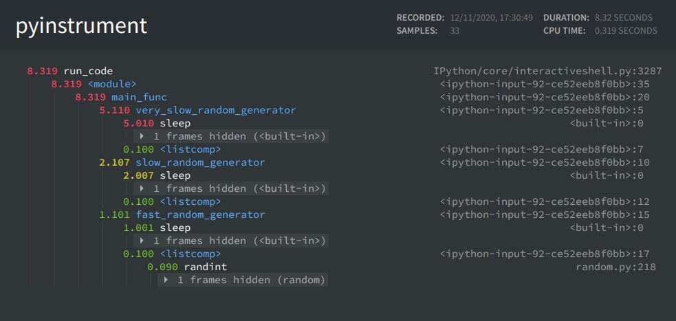
Below we have printed results in a text format using the timeline parameter as True. We have also explained the show_all parameter by setting it to True and then False later on.

print(profiler.output_text(color=True, show_all=False, timeline=True))
  _     ._   __/__   _ _  _  _ _/_   Recorded: 17:39:48  Samples:  33
 /_//_/// /_\ / //_// / //_'/ //     Duration: 8.320     CPU time: 0.316
/   _/                      v3.2.0

Program: /home/sunny/anaconda3/lib/python3.7/site-packages/ipykernel_launcher.py -f /home/sunny/.local/share/jupyter/runtime/kernel-c450ef03-3d9f-4980-8dc2-314d5fcbe1ae.json

8.316 run_code  IPython/core/interactiveshell.py:3287
`- 8.316 <module>  <ipython-input-116-ce52eeb8f0bb>:35
   `- 8.316 main_func  <ipython-input-116-ce52eeb8f0bb>:20
      |- 1.101 fast_random_generator  <ipython-input-116-ce52eeb8f0bb>:15
      |  |- 1.001 sleep  <built-in>:0
      |  |     [2 frames hidden]  <built-in>
      |  `- 0.100 <listcomp>  <ipython-input-116-ce52eeb8f0bb>:17
      |- 2.107 slow_random_generator  <ipython-input-116-ce52eeb8f0bb>:10
      |  |- 2.007 sleep  <built-in>:0
      |  |     [2 frames hidden]  <built-in>
      |  `- 0.100 <listcomp>  <ipython-input-116-ce52eeb8f0bb>:12
      `- 5.108 very_slow_random_generator  <ipython-input-116-ce52eeb8f0bb>:5
         |- 5.008 sleep  <built-in>:0
         |     [2 frames hidden]  <built-in>
         `- 0.100 <listcomp>  <ipython-input-116-ce52eeb8f0bb>:7


print(profiler.output_text(color=True, show_all=True, timeline=True))
  _     ._   __/__   _ _  _  _ _/_   Recorded: 17:39:48  Samples:  33
 /_//_/// /_\ / //_// / //_'/ //     Duration: 8.320     CPU time: 0.316
/   _/                      v3.2.0

Program: /home/sunny/anaconda3/lib/python3.7/site-packages/ipykernel_launcher.py -f /home/sunny/.local/share/jupyter/runtime/kernel-c450ef03-3d9f-4980-8dc2-314d5fcbe1ae.json

8.316 run_code  IPython/core/interactiveshell.py:3287
`- 8.316 <module>  <ipython-input-116-ce52eeb8f0bb>:35
   `- 8.316 main_func  <ipython-input-116-ce52eeb8f0bb>:20
      |- 1.101 fast_random_generator  <ipython-input-116-ce52eeb8f0bb>:15
      |  |- 1.001 sleep  <built-in>:0
      |  `- 0.100 <listcomp>  <ipython-input-116-ce52eeb8f0bb>:17
      |- 2.107 slow_random_generator  <ipython-input-116-ce52eeb8f0bb>:10
      |  |- 2.007 sleep  <built-in>:0
      |  `- 0.100 <listcomp>  <ipython-input-116-ce52eeb8f0bb>:12
      `- 5.108 very_slow_random_generator  <ipython-input-116-ce52eeb8f0bb>:5
         |- 5.008 sleep  <built-in>:0
         `- 0.100 <listcomp>  <ipython-input-116-ce52eeb8f0bb>:7


Sunny Solanki  Sunny Solanki

YouTube Subscribe Comfortable Learning through Video Tutorials?

If you are more comfortable learning through video tutorials then we would recommend that you subscribe to our YouTube channel.

Need Help Stuck Somewhere? Need Help with Coding? Have Doubts About the Topic/Code?

When going through coding examples, it's quite common to have doubts and errors.

If you have doubts about some code examples or are stuck somewhere when trying our code, send us an email at coderzcolumn07@gmail.com. We'll help you or point you in the direction where you can find a solution to your problem.

You can even send us a mail if you are trying something new and need guidance regarding coding. We'll try to respond as soon as possible.

Share Views Want to Share Your Views? Have Any Suggestions?

If you want to

  • provide some suggestions on topic
  • share your views
  • include some details in tutorial
  • suggest some new topics on which we should create tutorials/blogs
Please feel free to contact us at coderzcolumn07@gmail.com. We appreciate and value your feedbacks. You can also support us with a small contribution by clicking DONATE.


Subscribe to Our YouTube Channel

YouTube SubScribe

Newsletter Subscription