XGBoost - An In-Depth Guide [Python API]¶

> What is XGBoost (Extreme Gradient Boosting)?¶

Xgboost is a machine learning library that implements the gradient boosting algorithms (gradient boosted decision trees). The gradient boosted decision trees is a type of gradient boosting machines algorithm that has many decision trees in an ensemble. All these decision trees are generally weak predictors and their predictions are combined to make final prediction.

> Why Choose "XGBoost" Over Other Gradient Boosting Trees Implementations?¶

XGBoost is designed to be quite fast compared to the implementation available in sklearn.

XGBoost lets us handle a large amount of data that can have samples in billions with ease.

It can run in parallel and distributed environments to speed up the training process. The distributed algorithm can be useful if data does not fit into to main memory of the machine. Currently, it has support for dask to run the algorithm in a distributed environment.

Xgboost even supports running an algorithm on GPU with a simple configuration which will complete quite fast compared to when run on CPU.

Xgboost provides API in C, C++, Python, R, Java, Julia, Ruby, and Swift.

Xgboost code can be run on a distributed environment like AWS YARN, Hadoop, etc.

It even provides an interface (CLI) to run the algorithm from the command line/shell.

Apart from this, xgboost provides support for controlling feature interactions, custom evaluation functions, callbacks during training, monotonic constraints, etc.

> What Can You Learn From This Article?¶

As a part of this tutorial, we have explained how to use Python library XGBoost to solve machine learning tasks (Classification & Regression). We have explained majority of Python API with simple and easy-to-understand examples.

Apart from training models & making predictions, we have covered concepts like cross-validation, saving & loading models, visualizing features importances, early stop training to avoid overfitting, creating custom object/loss function, creating custom evaluation metrics, callbacks during training, distributed training using dask, GPU training, etc.

All our examples are trained on toy datasets (structured - tabular) available from scikit-learn to keep things simple and easy to grasp

We have tried to cover the majority of features available from xgboost to make this tutorial a short reference to master xgboost Python API.

> Which Other Python Libraries Provides Implementation Of Gradient Boosted Trees?¶

• CatBoost
• LightGBM
• Scikit-Learn

> How to Install XGBoost?¶

• PIP
  • pip install -U xgboost
• Conda
  • conda install py-xgboost

Below, we have listed important sections of tutorial to give an overview of the material covered. We know that the list below is big but you can skip some sections of tutorial which has a theory or repeat example of some concepts. We have included NOTE in those sections so you can skip them to complete tutorial faster. You can then refer to those sections in your free time or as per need.

Important Sections Of Tutorial¶

1. Load Datasets for Tutorial
   • Boston Housing Dataset
   • Breast Cancer Dataset
   • Wine Dataset
2. XGBoost Estimators at High-Level (High-Level API)
3. Core API: Booster Estimator
   • Booster: Regression Example
     • Divide Data into Train and Test Sets
     • DMatrix: XGBoost Data Structure to Represent Data
     • "train()": Train Model
     • "predict()": Make Predictions
     • Evaluate Model Performance
     • Visualize Features Importances using "plot_importance()"
   • Important Parameters of Boosting (train())
   • Booster: Tweedie Regression Example
   • Booster: Binary Classification Example
   • Booster: Multi-Class Classification Example
   • Saving and Loading Trained Model
   • Cross Validation
4. Sklearn Like API
   • XGBRegressor
     • Train Model, Make Predictions & Evaluate Model Performance
     • Hyperparameters Tuning using Grid Search
   • XGBClassifier
   • XGBRFRegressor
   • XGBRFClassifier
5. Early Stop Training to Avoid Overfitting
6. Feature Interaction Constraints
7. Monotonic Constraints
8. Custom Objective/Loss Function
9. Custom Evaluation Functions
10. Callbacks
11. Dask Backend for Distributed Training
12. GPU Support
13. GPU & Dask Together For Parallel GPUs

We'll start by importing the necessary libraries which we'll use as a part of this tutorial.

1. Load Datasets¶

We'll be using the below-mentioned three different datasets which are available from sklearn as a part of this tutorial for explanation purposes.

1. Boston Housing Dataset: It's a regression problem dataset which has information about a various attribute of houses in Boston and their price in dollar. This will be used for regression tasks.
2. Breast Cancer Dataset: It's a classification dataset which has information about two different types of tumor. It'll be used for explaining binary classification tasks.
3. Wine Dataset - It's a classification dataset which has information about ingredients used in three different types of wines. It'll be used for explaining multi-class classification tasks.

We have loaded all three datasets mentioned one by one below. We are printing descriptions of datasets which gives us an overview of dataset features and size. We have even loaded each dataset as a pandas data frame and displayed the first few samples of data.

Boston Housing Dataset¶

Breast Cancer Dataset¶

Wine Dataset¶

2. XGBoost Estimators at High-Level (High-Level API)¶

Below, we have listed important estimators provided by XGBoost to perform classification and regression tasks.

1. Booster - It's a universal estimator which can handle both classification and regression datasets with settings. We can create it by calling train() function of XGBoost library.
2. XGBRegressor - It is an estimator with scikit-learn like API designed to work with regression datasets.
3. XGBClassifier - It is an estimator with scikit-learn like API designed to work with classification datasets.
4. XGBRFRegressor - It is an estimator with scikit-learn like API and random forest implementation designed to work with regression datasets.
5. XGBRFClassifier - It is an estimator with scikit-learn like API and random forest implementation designed to work with classification datasets.

We'll now explain estimators one by one with examples.

3. Core API: Booster Estimator ¶

As a part of this section, we'll explain the core API of xgboost which will have an explanation for different machine learning estimators available with the library. We'll even explain the parameters of these estimators as well as important attributes and methods available through them.

3.1 Booster: Regression Example ¶

We'll start with the creation of a simple estimator for the regression task of predicting prices of houses in Boston. We'll explain how we can use API to create an estimator with default parameters which will just work fine. We'll then explain various parameters available for different purposes.

3.1.1 Divide Data into Train and Test Sets¶

We'll first divide Boston dataset into train (90%) and test (10%) datasets using sklearn's function train_test_split().

3.1.2 DMatrix: XGBoost Data Structure to Represent Data¶

Xgboost default API only accepts a dataset that is wrapped in DMatrix. DMatrix is an internal data structure of xgboost that wraps data features and labels both into it. It's designed to be efficient and fastens the training process.

We can create a DMatrix instance by setting a list of the below parameters. Only the data parameter is required and all others are optional.

• data - This parameter accepts one of the below as input which has values for data features.
  • pandas dataframe
  • numpy array
  • scipy sparse matrix
  • path to libsvm format text file
  • libsvm format text
• label - It accepts a numpy array of pandas data frame containing labels of the dataset.
• missing - It accepts float value in the dataset which should be treated as a missing value. The default is "None" meaning that "np.nan" is considered missing.
• feature_names - It accepts a list of string specifying feature names of data.
• feature_types - It accepts a list of string specifying feature data types.
• nthread - It accepts integer specifying the number of threads to use when loading data. The value of -1 uses all available threads on the system.

Below we have created train DMatrix and test DMatrix using numpy arrays of features data and labels. We have also passed feature names to the constructor.

3.1.3 "train()": Train Model¶

The simplest way of creating a booster using xgboost is by calling the train() method of xgboost. The train() method returns an instance of class xgboost.core.Booster after training is completed. We need to pass parameters for boosting algorithm as a dictionary to train method.

Below we have given a list of important parameters of the train() method. Only params and dtrain are required and all other parameters are optional and have default values set to them.

• params - It accepts a dictionary of gradient boosting algorithm parameters. We can give it an even empty dictionary and it'll take the default value for all parameters. By default, it'll consider the task to be a regression task and will calculate RMSE loss. We need to specify at least an objective function if we want it to consider a classification task for the data.
• dtrain - It accepts DMatrix instances of train data.
• num_boost_round - It accepts integer specifying the number of rounds of the training process. The algorithm will iterate over whole training data many times.
• evals - We can provide a list of tuples specifying datasets to be used for evaluation when performing training. We have passed our train and test datasets as evaluation sets hence RMSE for each will be printed after all iterations.
• obj - We can give customized objective function which will be maximized/minimized when training algorithm.
• feval - We can give a customized evaluation function that will be used to evaluate datasets given to evals.
• maximize - It accepts a boolean specifying whether to maximize or minimize our objective/loss function.
• early_stopping_rounds - It accepts an integer that instructs the algorithm to stop training if the last eval set in the list has not improved for that many rounds. If the objective/loss of the last eval dataset has not improved for that many consecutive rounds of training then the training process will stop. This parameter requires us to provide an evals parameter for it to work.
• evals_result - We can provide an empty dictionary to this parameter and it'll store evaluation results in it.
• verbose_eval - It accepts bool or integer specifying whether to print evaluation results. The integer value greater than 0 will print evaluation results at every that many iterations.
• callbacks - It accepts a list of callbacks that are applied at the end of each iteration of the training process.

Below we have called the train() method of xgboost by passing it a few parameters for boosting algorithm, train data for training, and evaluation set of training and test dataset on which evaluation after each iteration will happen.

3.1.4 "predict()": Make Predictions¶

We can use the predict() method of booster instance to predict labels for data passed to it. The predict() method requires us to pass the DMatrix instance only.

The predict method provides a list of the below important parameters that can be useful in different situations.

• data - It accepts DMatrix of feature values.
• ntree_limit - It accepts an integer specifying the number of trees to use from the total tree to make a prediction. The default is 0 which means to use all trees.
• pred_leaf - It accepts boolean which is set to True returns array of size n_samples x n_trees where each entry is an index of leaf in a tree which was used for prediction. The entry (0,1) refers to an index of leaf for the 2nd tree which was used to make a prediction for the first sample. The default is False.
• pred_contribs - It accepts boolean which if set to True returns an array of size n_sample x n_features+1 where each entry specifies contributions of features in making a final prediction for that sample. It's referred to as SHAP values. If we add all values for a particular sample then we can get the actual prediction. The default is False.
• pred_interactions - It accepts boolean which if set to True returns array of size n_sample x n_features+1 xn_features+1 indicating features SHAP interaction values for each sample.

Below we have created a data frame showing the first 10 actual test labels and 10 predicted labels for test data.

Below we have retrieved shap values for our test samples. We have even summed up shap values for each sample to calculate the final prediction which is the same as the actual prediction printed above.

If you are interested in learning about the SHAP python library which provides various methods for calculating SHAP values and different types of plots to interpret them then please feel free to check our tutorial on the same.

• SHAP - Explain Machine Learning Model Predictions using Game-Theoretic Approach

3.1.5 Evaluate Model Performance¶

We can explicitly evaluate the dataset using a trained booster instance with the help of the eval() method. It'll evaluate the dataset and return an objective function value for it. below we are using the eval() method on the train and test DMatrix to get RMSE for both.

Below we have evaluated the R2 score for train and test datasets using the r2_score() function of sklearn. We have then evaluated the R2 score based on using only 5 trees from the ensemble rather than using all trees.

Scikit-learn provides many commonly used machine learning metrics for evaluating model performance on regression, classification, and clustering tasks. Please feel free to check below link if you want to learn about them.

• Scikit-Learn: Model Evaluation Metrics/Scoring Functions

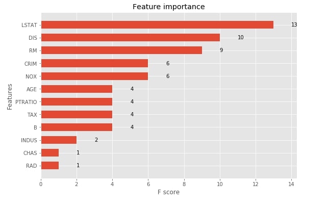
3.1.6 Visualize Features Importances using "plot_importance()"¶

The xgboost provides functionality that lets us print feature importance. We need to pass our booster instance to the method and it'll plot feature importance bar chart using matplotlib. The plot_importance() method has an important parameter named importance_type which accepts one of the below-mentioned 3 string values to plot feature importance in three different ways.

• weight - It plots the number of times a feature appears in a tree. This is the default value.
• gain - It plots the average gain of splits that uses the feature.
• cover - It plots the average coverage of splits for each feature.

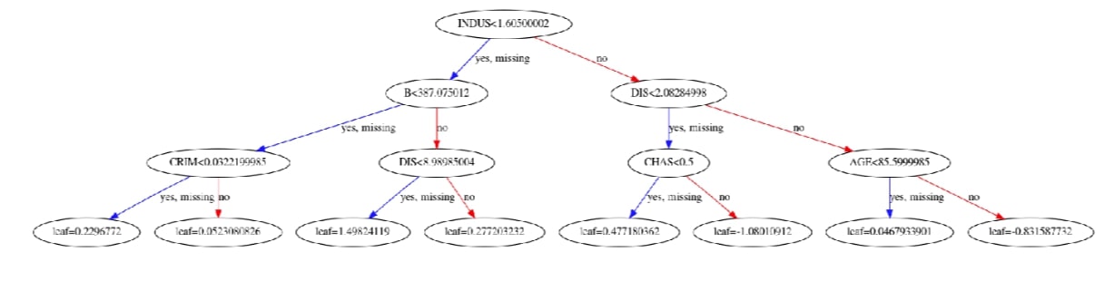
Visualize Individual Boosted Tree using "plot_tree()"¶

Xgboost also lets us plot the individual trees in the ensemble of trees using the plot_tree() method. It accepts booster instance and index of a tree which we want to plot. Below we have plotted the 10th tree of an ensemble. Please make a note that indexing starts at 0.

Visualize Feature Values Split Histogram using "get_split_value_histogram()"¶

The get_split_value_histogram() method returns histogram of splits for feature values. Below we have created split values histogram for feature LSTAT of data. It gives us value and how many times a split has happened at that value.

Convert Trees to Dataframe using "trees_to_dataframe()"¶

The trees_to_dataframe() method will dump information on trees used in an ensemble as a pandas dataframe. It'll have information on each tree-like individual node ids, feature name, and its values used for a split at each node, gain at each node, cover at each node, etc.

3.2 Important Parameters of Boosting (train()) ¶

NOTE: Please feel free to skip this section if you are in hurry. It is a theoretical section listing parameters of "train()" function. You can refer to them later as you need to tweak model.

Below we have given a list of important parameters of the boosting algorithm which we can pass as a dictionary to the params parameter of "train()" function as well as other XGBoost models (XGBRegressor, XGBClassifier, etc) explained below.

• booster - It specifies which gradient boosting algorithm to use for training. Below is a list of possible options.
  • gbtree - It’s a tree-based algorithm. Default.
  • gblinear - It’s a linear function based algorithm.
  • dart - It’s a tree-based algorithm.
• eta - It accepts float [0,1] specifying learning rate for training process. Default = 0.3

• tree_method - It accepts string specifying tree construction algorithm. Below is a list of possible options.

  • auto - It automatically decides the algorithm based on dataset size. For the small datasets, it uses exact and for larger datasets approx.
  • exact - It specifies the exact greedy algorithm. It tries all possible splits to create trees.
  • approx - It’s an approximate greedy algorithm that uses quantile sketch and gradient histogram.
  • hist - It’s an approximate greedy algorithm optimized using a faster histogram.
  • gpu_hist - Its a GPU implementation of hist.

• max_depth - It accepts an integer specifying the maximum depth of the tree. The default is 6.

• gamma - It accepts float specifying minimum loss required to make a further partition on a particular node of the tree during training. The default is 0.
• subsample - It accepts float in the range (0,1] specifying sub-sample ratio of training samples. The value of 0.5 will result in taking half of the sample randomly before training starts which can help prevent overfitting.

• sampling_method - This parameter accepts one of the below string as a sampling method to draw sub-samples.

  • uniform - Default
  • gradient_based

• lambda - It accepts float specifying L2 regularization term on weights. The default is 1.

• alpha - It accepts float specifying L1 regularization term on weights. The default is 0.
• max_bin - It accepts an integer specifying the number of bins to bucket continuous features. The default is 256. The more value improves split quality at the expense of more computation time.
• monotone_constraints - It accepts tuple of integers of length n_features. Each entry in tuple has a value of either 1,0 or -1 specifying increasing, none, or decreasing monotone relation of a feature with the target. It only works with tree_method set to one of the exact, hist or gpu_hist.
• interaction_constraints - It accepts a list of the list each individual list represents indexes of features that are allowed to interact when creating a tree to make the final prediction. If we don't provide this constraint then all features are allowed to interact with one another. We can restrict feature interaction using this parameter.
• tweedie_variance_power - It accepts float in the range (1,2) that controls variance of Tweedie distribution. The default value is 1.5.

• objective - It accepts string specifying objective/loss function to use for training. The default value is reg:squarederror. Below are some of the commonly used values. Please visit this link to check a list of all objective functions available.

  • reg:squarederror
  • reg:squaredlogerror
  • reg:logistic - Logistic Regression
  • binary:logistic - Logistic Regression for Binary Classification. Outputs probability.
  • multi:softmax - Multi-Class classification using softmax function.
  • multi:softprob - It’s the same as softmax but outputs probability.
  • reg:tweedie - It’s tweedie regression with log-link.

• eval_metric - It accepts string value specifying metric which will be used to evaluate evaluation sets passed to evals parameter. Below is a list of commonly used values. Please visit this link to check a list of all evaluation metrics available.

  • rmse - Root Mean Squared Error
  • rmsle - Root Mean Squared Log Error
  • mae - Mean Absolute Error
  • logloss - Negative Log-likelihood
  • auc - Area Under Curve ROC
  • error - Binary Classification error rate (no_wrong_preds/total_samples).
• num_class - It's an integer specifying number of class for multi-class classification problem. We need to provide this when the objective is set to multi:softmax or multi:softprob.
• nthread - It specifies the number of threads to use to run xgboost.
• verbosity - It accepts one of the below integers for printing messages during training.
  • 0 - Silent
  • 1 - Warning
  • 2 - Info
  • 3 - Debug

Please make a NOTE that this is not a list of all parameters for estimator but a list of important parameters that are commonly tuned by practitioners. Please visit the below link to know about all possible parameters available with xgboost.

• XGBoost Important Parameters

3.3 Booster: Tweedie Regression Example ¶

NOTE: Please feel free to skip this section if you are in hurry and have understood how to perform regression from previous section. It is explaining usage of different objective/loss function.

Below we have explained an example of how we can use tweedie regression on Boston housing data. We have trained the model using tweedie regression and then evaluated RMSE and R2 scores on both train and test datasets.

3.4 Booster: Binary Classification Example ¶

As a part of this section, we have explained how we can use the train() method to train booster for the binary classification task of classifying breast cancer tumor types. Please make a note that we have used binary:logistic as our objective function hence the output of the predict() method of the booster will be a probability. We have included logic to convert probabilities into class. We have then calculated accuracy, confusion matrix, and classification report for test data.

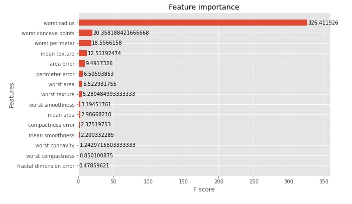
Below we have plotted feature importance for booster trained on breast cancer dataset. We have plotted the average gain of splits that uses the feature. Please feel free to look at the data frame retrieved using the trees_to_dataframe() method.

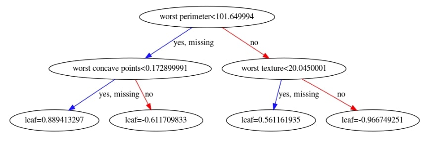
We have now plotted 3rd tree from the ensemble below.

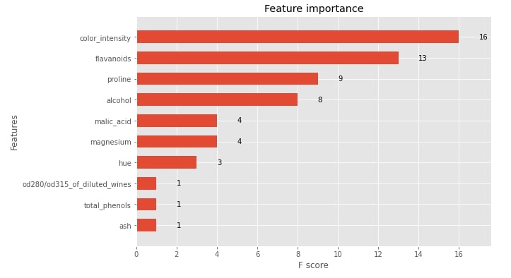
3.5 Booster: Multi-Class Classification Example ¶

NOTE: Please feel free to skip this section if you are in hurry and have understood how to perform classification from previous binary classification section.

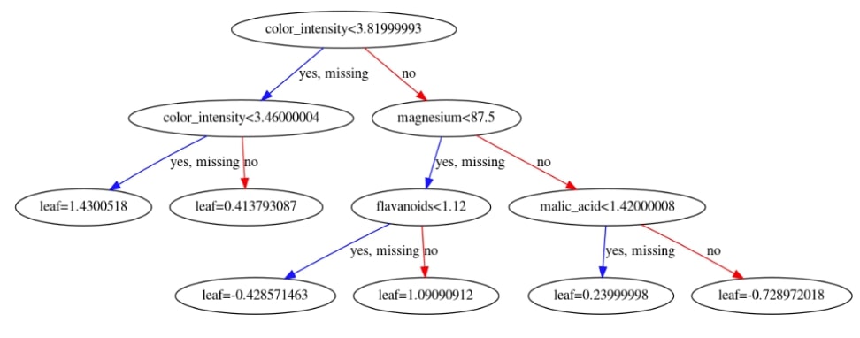
As a part of this section, we have explained how we can use the train() method for multi-class classification problems. We have used it to generate booster trained on wine classification train dataset. We have then evaluated the accuracy, confusion matrix, and classification report on the test dataset.

We have then plotted the feature importance bar chart and first decision tree.

3.6 Saving and Loading Trained Model ¶

As a part of this section, we have explained how we can save the trained xgboost model to disk and then load it to make predictions again in the future.

Below is a list of available methods that can be used to save the model in a different format.

• save_model(file_name) - It saves model in xgboost internal format.
• save_config() - It outputs booster configuration as JSON string which can be saved to json file. We can load the booster later using the same parameter configuration using this file.
• save_raw() - It returns the byte array object which is the current memory representation of a booster instance.

Below is a list of available methods that can be used to load the saved model.

• load_model(file_name) - It accepts file name or byte array from which trained model can be loaded.
• load_config() - It accepts JSON string generated by save_config() to load model with same configuration.

Below we have saved our multi-class classification model which we created in the previous example. We have then reloaded the model and made predictions using it for verification.

We can even load the model by using the Booster() class giving it the file name as a part of the model_file parameter.

3.7 Cross Validation ¶

Xgboost lets us perform cross-validation on our dataset as well using the cv() method. The cv() method has almost the same parameters as that of the train() method with few extra parameters as mentioned below.

• nfold - It accepts an integer specifying the number of folds to create from the dataset. The default is 3.
• folds - It accepts sklearn KFold, StratifiedKFold, ShuffleSplitor StratifiedShuffleSplit instance.
• metrics - It accepts list of metrics to evaluate.

Below we have performed cross-validation on the full Boston dataset for 10 rounds and 5 folds.

Below we have again performed cross-validation on the Boston dataset but this time we have passed sklearn ShufflSplit for creating folds. It creates 10 fold of randomly shuffled data.

Below we have performed cross-validation on the breast cancer dataset. We have informed the cv() method to evaluate log loss, AUC, and error metrics for each iteration.

4. Sklearn Like API ¶

Xgboost provides estimators that have almost the same API like that of sklearn estimators. This helps developers with sklearn background to grasp the usage of xgboost faster. It even lets us use the xgboost model with sklearn's grid search functionality. As a part of this section, we'll explain 4 estimators available from xgboost which has the same API as sklearn's estimators.

• XGBRegressor
• XGBClassifier
• XGBRFRegressor
• XGBRFClassifier

4.1 XGBRegressor ¶

The XGBRegressor is an estimator that is used for regression problems. It has a default objective function as reg:squarederror. It has a list of parameters that we gave as a dictionary to the train() method. We pass those parameters to the constructor of XGBRegressor directly.

4.1.1 Train Model, Make Predictions & Evaluate Model Performance¶

Below we have trained XGBRegressor on Boston train data and then calculated R2 score on test and train dataset both. The score() method is available as a part of estimators which has sklearn like API. The score() method will return the R2 score for regression tasks and accuracy for classification tasks.

Below we have printed the number of estimators which model used by default, max depth of each tree, and feature importance of individual features.

4.1.2 Hyperparameters Tuning using Grid Search¶

We have now explained how we perform a grid search with XGBRegressor. We have tried different values of parameters n_estimators, max_depth, and eta to find the best performing values. We have then plotted grid search results as well.

4.2 XGBClassifier ¶

The XGBClassifier is an estimator that is used for classification tasks. It has the default objective function binary:logistic. We can pass the same parameters which we can pass to the train() method's params parameter as a dictionary to the constructor of XGBClassifier. We can get actual predictions using predict() method and probabilities using predict_proba() method. It even provides a score() method which lets us calculate the accuracy of the model on given data.

4.2.1 Train Model, Make Predictions & Evaluate Model Performance¶

Below we have trained XGBClassifier on the breast cancer train dataset. We have then evaluated accuracy on train and test datasets. We have also printed the first few predictions and probabilities.

4.2.2 Hyperparameters Tuning using Grid Search¶

Below we have explained how we can use XGBClassifier with sklearn's grid search functionality to try a list of parameters to find the best parameter settings.

4.3 XGBRFRegressor ¶

4.3.1 Train Model, Make Predictions & Evaluate Model Performance¶

The XGBRFRegressor is a random forest implementation based on decision trees for regression tasks. It has almost exactly the same API as that of XGBRegressor. We have explained below the usage of it on the Boston housing dataset.

4.3.2 Hyperparameters Tuning using Grid Search¶

4.4 XGBRFClassifier ¶

4.4.1 Train Model, Make Predictions & Evaluate Model Performance¶

The XGBRFClassifier is a random forest implementation based on decision trees for classification tasks. It has almost exactly the same API as that of XGBClassifier. We have explained below the usage of it on the breast cancer dataset.

4.4.2 Hyperparameters Tuning using Grid Search¶

5. Early Stop Training to Avoid Overfitting ¶

Xgboost provides us with an option that lets us stop the training process if training loss is not improving for some specified number of iterations. We can specify the early_stopping_rounds parameter in the train() method to some integer and it'll stop training if training loss is not improved for that many rounds of training.

Below we have instructed train() method to train for 20 rounds using num_boost_round parameter and early_stopping_rounds is set to 5. The train() method will stop training if training loss is not improved for 5 sequential rounds of training.

We have below explained how we can early stop training with XGBRegressor.

6. Feature Interaction Constraints ¶

When xgboost creates a tree during the training process it takes into consideration all feature interactions. In a decision tree, we have nodes where each node represents a decision to be made based on a particular value of the feature. The next node will be based on the feature value mentioned in the previous node. By default, all features can be present in any node of the decision tree. We can force xgboost to keep a list of features in subsequent nodes by giving it a list of indices of features in the dataset. We can give list of list to interaction_constraints parameter of train() method. Here an individual list is a list of feature indices that should only interact with one another and not with other features.

Please feel free to go through this link to get in-depth details about feature interaction constraints in xgboost.

Below we have kept features 0,1,2,11 and 12 into one list hence these features will interact with one another when creating a tree but not with other features hence tree will have only these features. The Same goes for other lists.

Below we have explained how we can use feature interaction constraint with XGBRegressor.

7. Monotonic Constraints ¶

The monotonic constraints let us specify increasing, decreasing, or no monotone relation of the feature with the target. We can specify a monotone value of 1,0 or -1 for each feature to show the increasing, none, and decreasing relation of the feature with the target by setting the monotone_constraints parameter. Below we have explained the usage of monotonic constraints for regression problems using the Boston dataset.

Please feel free to check this link to better understand monotonic constraints.

8. Custom Objective/Loss Function ¶

As a part of this section, we have explained how we can use a custom objective/loss function with xgboost. We'll be giving input to loss function list of predicted values and actual target values. It'll then return a list of the first derivative and second derivative of loss function for that values. Below we have created the mean squared error loss function and explained its usage with a simple example. We need to pass a reference to function to the objective parameter of an estimator.

9. Custom Evaluation Functions ¶

Xgboost lets us create our custom evaluation function as well. The function should accept predictions and DMatrix instances as parameters and then calculate metrics based on predictions and actual target values. We have created simple mean_absolute_error() for explanation purpose.

We can pass function reference to the feval parameter of train() to use it on the evaluation dataset.

Below we have explained how we can use custom evaluation metrics with XGBRegressor. We need to set the eval_metric parameter of the fit() method with reference to the custom evaluation function.

10. Callbacks ¶

Xgboost provides us with a list of callback functions for a different purpose which gets executed after each iteration of training. Below is a list of available callbacks with xgboost as a part of the callback module.

• early_stop - It accepts integer specifying whether to stop training if evaluation metric results on last evaluation set are not improved for that many iterations.
• print_evaluation - It accepts integer values specifying how often to print evaluation results. Evaluation metric results are printed at every that many iterations as specified.
• record_evaluation - It accepts a dictionary in which evaluation results will be recorded.
• reset_learning_rate - It lets us reset the learning rate after each iteration of training. It accepts an array of size the same as the number of iterations or callback returning the new learning rate for each iteration.

We need to provide a list of callbacks to the callbacks parameter for their execution after each iteration.

Below we have explained usage of early_stop(), print_evaluation() and record_evaluation() callbacks for regression task.

Below we have again explained the same three callbacks with XGBRegressor. This time we need to pass a list of callback functions to the callbacks parameter of the fit() method.

As a part of this example, we have explained how we can use the reset_learning_rate() callback. We have first called the reset_learning_rate() function with an array of size 15 which is the same as the number of iterations of our training process. The array starts from 0.1 till 1.5 increasing the learning rate by 0.1 each time.

We have now explained another example demonstrating usage of the reset_learning_rate() callback. This time we have created a function named calculate_learning_rate() which will be passed to reset_learning_rate() callback. The function takes as input two integers (current boosting round index and a total number of boosting rounds) and returns the learning rate for that boosting round. We have then passed the callback created to the callbacks parameter.

11. Dask Backend for Distributed Training Of XGBoost Models ¶

Xgboost provides support for using dask as a backend for training gradient boosting algorithm in a distributed environment. Xgboost has a module named dask which has a list of data structures and estimators for using with dask.

Dask has a simple structure where we have below mentioned three main components.

• Scheduler - Dask distributed environment has one scheduler which handles communication between clients and workers. It’s even responsible for distributing work to worker nodes.
• Clients - We can have more than one client instances which can be used to submit tasks to the scheduler.
• Workers - These are actual nodes(processes/machines) which runs task.

In order to use dask, we need to create a client that will be used to communicate with the scheduler. This tutorial is run on a single PC and not on a distributed environment with multiple nodes. When we create an instance of dask client without giving the IP address and port of scheduler, it'll create a cluster on the local machine itself. Below we have created a small cluster of 4 workers using the Client() constructor.

If you are interested in learning about dask then please feel free to check our tutorials on the same. It has information about creating a dask distributed environment as well on an actual cluster with multiple machines.

• dask.distributed - Parallel Processing in Python
• dask.delayed - Parallel Computing in Python
• dask.bag - Parallel Computing in Python

Please make a note that using xgboost on the dask distributed environment requires a little background of dask to make it work correctly.

Below we have divided the Boston housing dataset into the train (90%) and test (10%) sets. We have then converted the normal numpy array to the dask array using the da module of the xgboost.dask module. The da module provides access to the dask.array module. We can even use the dask.array module to create arrays and it'll work fine. The xgboost estimators are available through the xgboost.dask module accepts either the dask array or dask dataframe. The dask.dataframe module is available in xgboost as xgboost.dask.dd.

Please feel free to check below links if you are looking for some guidance on dask.array and dask.dataframe.

• dask.array: Guide to Work with Large Arrays in Parallel
• dask.dataframe: Simple Guide to Work with Large Tabular Datasets

Below we have explained how we can run the xgboost algorithm in a dask distributed environment. The dask module has its own DaskDMatrix data structure which is almost the same as DMatrix but requires client instance as the first argument followed by data arrays containing features values and target labels.

The train() method available through the dask module requires us to pass the client instance first before the parameters dictionary. Everything else is the same as the train() method available directly. It runs training in a distributed environment and returns a dictionary with two components (Booster instance and training history). We can then call the predict() method of the dask module by giving it the client, booster instance, and DaskDMatrix dataset. It'll return a lazy instance on which we need to call compute() to evaluate it and return the actual result. We have calculated the R2 score on train and test datasets at last.

Below we have explained how we can use the DaskXGBRegressor() estimator for regression task with the Boston housing dataset. It has the same API as that of XGBRegressor(). We have first created a client instance and then used it as context to call all other methods which will require the usage of dask distributed environment.

As the last example of using xgboost with dask, we have explained how we can use the DaskXGBClassifier() estimator for classification tasks. The majority of things are almost the same as normal API with differences like using the client to communicate to dask cluster, wrapping data into dask data structures, and calling compute() on lazy instances to actually run a task on a cluster to get results.