Dask DataFrames: Simple Guide to Work with Large Tabular Datasets
In this age of data, tabular datasets are one of the most common datasets that data scientists encounter. The majority of organizations store data in tabular format in a database or in some other format. Python provides a wonderful library named pandas for working with tabular datasets. It has a wide API that lets us perform a bunch of operations with tabular datasets. It's the first choice of the majority of developers when working with tabular data.
Though pandas is widely accepted, it has some limitations. The size of the real-world datasets is growing day by day and many real-world datasets generally do fit into the main memory (RAM) of the computers. Pandas can only handle datasets that fit into the main memory of the computer. There are situations where the dataset is too large to fit into the main memory and in this kind of situation pandas can not be used to perform data analysis.
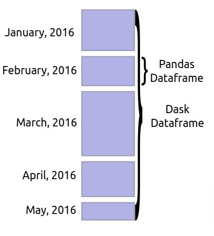
To solve this problem, the dask developers developed wrappers around pandas which let us work on tabular datasets in chunks. Dask is one of the most famous distributed computing libraries in the python stack which can perform parallel computations on cores of a single computer as well as on clusters of computers. The dask dataframes are big data frames (designed on top of the dask distributed framework) that are internally composed of many pandas data frames. The datasets handled by dask data frames can be on a single computer or they can be scattered across clusters and dask will handle them. Dask dataframes does not load total data into memory and keeps only a lazy reference to data frames. All the operations performed on dask dataframes will be lazy and only operation details will be stored. The actual calculation will happen only when we call compute() method on the last reference that we got after performing all operations. Until we call compute() on the dataframe, the dask will only record operations and won't actually execute them. The call to compute() will inform dask to execute all operations performed on the dataframe which it'll then execute in parallel on clusters.
As a part of this tutorial, we'll explain how we can work with dask dataframes with simple examples. We won't be covering the dask distributed framework in detail here though. If you are interested in learning about the dask distributed framework then please feel free to check our below tutorials. It'll help you with this tutorial as well.
- dask.distributed - Parallel Processing in Python
- dask.delayed - Parallel Processing in Python
- dask.bag - Parallel Programming in Python
- dask - Global Variables, Queues, Locks & Publish/Subscribe
Below we have highlighted important sections of the tutorial to give an overview of the material that we'll be covering in this tutorial. We do have two extra small sections which are not listed below. One of them is creating a dask cluster and another is creating data for our tutorial.
Important Sections of Tutorial
- Read DataFrames & Few Simple Operations
- Set DateTime Index
- Repartition Dask DataFrame
- Save to Disk and Reload
- Map a Function on Partitions
- Filter Rows/Columns
- Create New Columns and Modify Column Data
- Common Statistics
- Resampling
- Rolling Window Function
- GroupBy Operation
- Plotting
Install Dask
We can install dask using the below commands. It'll install dask dataframes as well.
- python -m pip install "dask[complete]"
- pip install dask[complete]
We'll start by importing dask and dask.dataframe libraries.
import dask

print("Dask Version : {}".format(dask.__version__))
from dask import dataframe as dd
Create Dask Cluster (Optional)
In order to use dask, we'll be creating a cluster of dask workers. This is not a compulsory step as we can continue working with dask dataframes without creating dask clusters. But we are creating it to limit memory usage and the number of workers. This cluster also gives us a URL of the dashboard which dask provides to analyze parallel processing it performs behind the scenes. This can help us better understand operations and the time taken by them. The dask cluster we have created below is on a single computer but the dask cluster can be spread across clusters of computers as well.
If you want to know in detail about dask clusters then please feel free to check our below tutorial which explains the architecture of dask along with the cluster creation process.
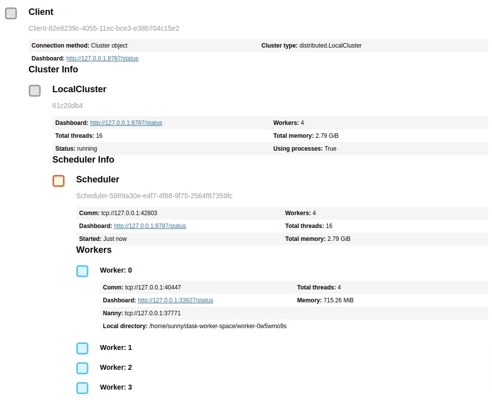
Below we have created a dask cluster of 4 processes where each process can use 0.75 GB of main memory. We can open the dashboard URL in a separate tab to see the progress of tasks when we execute some tasks on the dask cluster by calling compute() method.
from dask.distributed import Client

client = Client(n_workers=4, threads_per_worker=4, memory_limit='0.75GB')

client
Create Datasets
In this section, we have written small code to create datasets for our tutorial. We'll be creating a dataset with entries for each second of data from 1st Jan, 2021 to 28th Feb 2021. The data will be spread across separate CSV files where the CSV file for each day of the month will have entries for each second of the day. We'll be recording timestamp and 5 columns with random data in each CSV file. We have also created one categorical column in data which we'll be using when doing group-by operations on dataframes. We have stored all CSV files in a folder named dask_dataframes. There will be 31 CSV files for January month and 28 CSV files for February month.
import pandas as pd
import numpy as np

jan_2021 = pd.date_range(start="1-1-2021", end="2-28-2021")

for dt in jan_2021:
    ind_day = pd.date_range(start="%s 0:0:0"%dt.date(), end="%s 23:59:59"%dt.date(), freq="S")
    data = np.random.rand(len(ind_day), 5)

    cls = np.random.choice(["Class1", "Class2", "Class3", "Class4","Class5"], size=len(ind_day))

    df = pd.DataFrame(data=data, columns=["A", "B", "C", "D", "E"], index=ind_day)
    df["Type"] = cls

    df.to_csv("dask_dataframes/%s.csv"%dt.date())
!ls dask_dataframes/
Below we have loaded the first CSV file using pandas and displayed a few rows of it. In the next cell, we have loaded the last CSV file and displayed the last few rows of it to verify data.
import pandas as pd

df = pd.read_csv("dask_dataframes/2021-01-01.csv", index_col=0)

df.head()
df = pd.read_csv("dask_dataframes/2021-01-31.csv", index_col=0)

df.tail()
1. Read DataFrames & Simple Operations 
In this section, we'll explain how we can read big dataframes using dask.dataframe module and perform some basic operations on dataframe like setting index, saving dataframe to disk, repartition dataframe, work on partitions of dataframe individually, etc.
The dask.dataframe module provides us with method named read_csv() like pandas dataframe which we can use to read CSV files. It let us read one big CSV file or bunch of CSV files using unix pattern. We can use wildcard operator '*' to select and read more than one csv files.
- read_csv(urlpath, blocksize='default',sample=256000,sample_rows=10,**kwargs)
- This method takes as input a single string specifying a single file name or Unix file matching pattern specifying more than one file and returns an instance of dask.dataframe.Dataframe. We can also provide more than one file name as a list. This method returns immediately as it won't be reading all the files. It just returns a lazy reference to it. The actual data will only get read when we call compute() on the dataframe.
- The blocksize parameter accepts a string or integer specifying the block size of one block of data. The dask cuts large files into small pandas dataframes based on this block size. We can specify integer count specifying block size in bytes as 128,000,000 or we can specify as a string like '128MB'.
- The sample parameter accepts integer values specifying the number of bytes to read to determine the dtype of columns.
- This method also accepts majority of parameters which pandas read_csv() method accepts. Reference
Below we have read all files which are of month January using read_csv() method. We have provided a pattern with a wildcard to specify all files for January month. We have provided column names separately and instructed to skip the first row as it'll contain column names. We have also provided parse_date parameter which will be used to treat date column as datetime data type.
When we run the below cell, it returns immediately as it does not actually read all files. It'll read all files only when we call compute() method on an instance of dask.dataframe.DataFrame.
We can notice from the result getting displayed that it is displaying data type of columns and number of partitions of data. The npartitions specifies in how many partitions our data is divided and we'll explain how we can repartition our dataframe later in the tutorial. Here, the number of partitions is 31 because we had 31 CSV files for January month.
jan_2021 = dd.read_csv("dask_dataframes/2021-01-*.csv",
                       names=["date", "A", "B", "C", "D", "E", "Type"],
                       skiprows=1,
                       parse_dates=["date",]
                      )

jan_2021
Below we have called commonly used head() and tail() methods on the dataframe to look at the first and last few rows of data. The head() call will read only the first partition of data and tail() will read only the last partition of data for display.
Please make a NOTE that these two methods internally call compute() method to read data.
jan_2021.head()
jan_2021.tail()
We can access attributes like dtypes to retrieve data type of columns.
jan_2021.dtypes
The partitions attribute of the dask dataframe holds a list of partitions of data. We can access individual partitions by list indexing. The individual partitions themselves will be lazy-loaded dask dataframes.
Below we have accessed the first partition of our dask dataframe. In the next cell, we have called head() method on the first partition of the dataframe to display the first few rows of the first partition of data. We can access all 31 partitions of our data this way.
jan_2021.partitions[0]
jan_2021.partitions[0].head()
1.1 Set DateTime Index
In this section, we have set our date column as an index of our dask dataframe. We can set date column as index using set_index() method the same way we use it in pandas.
This dask operation is a little expensive and can take time in real life as it might need to shuffle entries of the dataframe.
The set_index() method returns a new modified dataframe and does not modify the dataframe in place. We have stored the new dask dataframe with date column as an index in a separate python variable.
We'll be using original integer indexed and this datetime indexed dataframes alternatively to explain various operations on dask dataframe in our tutorial.
jan_2021_new = jan_2021.set_index("date")

jan_2021_new
jan_2021_new.head()
Below we have read all files for February month using read_csv() file method. We have used a unix-like file matching pattern the same way we had used for reading all January month files. We'll be using this dataframe for explaining a few operations in our tutorial.
feb_2021 = dd.read_csv("dask_dataframes/2021-02-*.csv",
                       names=["date", "A", "B", "C", "D", "E", "Type"],
                       skiprows=1,
                       parse_dates=["date",]
                      )

feb_2021
Set DateTime Index
Below we have set date column as an index of the February month dask dataframe.
feb_2021_new = feb_2021.set_index("date")

feb_2021_new
feb_2021_new.head()
1.2 Repartition Dask DataFrame
In this section, we'll explain how we can repartition dask dataframes. When tasks are distributed on the dask cluster it generally works on partitions of dask dataframes in parallel. If partition size is quite big then it can slow down parallel operations. It's suggested in dask best practices that a single partition of the dask dataframe should hold 100 MB of data for good performance. After we have repartitioned the dask dataframe, when we try to save the dataframe, it'll create one file per partition which will be according to new partitions.
We can access a number of partitions of the dask dataframe by accessing npartitions attribute on the dataframe. We can also access the start index of each partition using divisions attribute of the dask dataframe. This can help us make better decisions on how to repartition the dataframe.
jan_2021.npartitions
print("Divisions : {}".format(jan_2021_new.divisions))
The dask dataframe provides us with a method named repartition() which can be used to repartition our dask dataframe. We can repartition the dask dataframe in various ways using different parameters of repartition() method. Below we have included the signature of repartition() method for explanation purposes.
- repartition(divisions=None,npartitions=None,partition_size=None,freq=None) - This method resizes dask dataframe according to new partitioning scheme specified using its parameter and returns repartitioned dask dataframe.
- The npartitions accept integer values specifying the number of partitions. It'll repartition the dask dataframe into a number of equal-sized partitions specified using this parameter.
- The divisions parameter accepts a list of index values specifying the start index of each partition.
- The partition_size parameter accepts integer or string values specifying partition size. The integer value is given then each partition will have that many bytes of data. The string value can be used to specify partition size like '10MB', '20KB', etc.
- The freq parameter is used when index of data is datetime index. We can specify freq strings like '1D', '24h', '15D', etc.
Below we have repartitioned our original dask dataframe from 31 partitioned dataframe to 50 partitioned dataframe using repartition() method. We have used npartitions parameter for this.
jan_2021_repartitioned = jan_2021.repartition(npartitions=50)

jan_2021_repartitioned
Below we have repartitioned our date indexed dask dataframe into 5 partitioned dataframe from 31 partitioned dataframe. We have used divisions parameter this time to repartition the dataframe. We have tried to repartition the dataframe into a new dataframe with each partition holding 7 days’ data. The last partition will have data for less than 7 days.
jan_2021_repartitioned_seven_days = jan_2021_new.repartition(divisions=[pd.Timestamp('2021-01-01 00:00:00'),
                                                             pd.Timestamp('2021-01-08 00:00:00'),
                                                             pd.Timestamp('2021-01-15 00:00:00'),
                                                             pd.Timestamp('2021-01-22 00:00:00'),
                                                             pd.Timestamp('2021-01-29 00:00:00'),
                                                             pd.Timestamp('2021-01-31 23:59:59')
                                                            ])

jan_2021_repartitioned_seven_days
Below we have repartitioned our datetime indexed dask dataframe where each partition holds 1H of data.
jan_2021_repartitioned_by_freq = jan_2021_new.repartition(freq="1H")

jan_2021_repartitioned_by_freq
1.3 Save to Disk and Reload
In this section, we'll explain how we can save the dask dataframe to files and reload them. We'll be saving files in CSV formats.
We can save dask dataframe to CSV files using to_csv() function. It works exactly like the pandas to_csv() method with the only difference that it'll create one CSV file for each partition of data.
Below we have saved our repartitioned dask dataframe to a folder named JAN_2021. We have provided filename as 'JAN_2021/*.csv'. Internally, dask runs a counter and gives file names according to that counter.
In the next cell, we have printed the contents of the directory JAN_2021. We can notice that it has 50 CSV files as we had saved our 50 partitioned dataframe to it.
file_names = jan_2021_repartitioned.to_csv("JAN_2021/*.csv", index=False)
!ls JAN_2021
Below we have reloaded all CSV files from JAN_2021 folder using read_csv() method.
jan_2021_reloaded = dd.read_csv("JAN_2021/*")

jan_2021_reloaded
Below we have created another example where we have explained how we can create a function to create file names for individual CSV files when saving them if we don't like default integer counter-based naming.
We can give a function to a parameter named name_function which takes a single parameter as input and returns a string specifying a filename. The dask will give incremental counter value to this function and it'll create a filename around counter value.
Below we have saved our repartitioned dask dataframe to JAN_21 folder. We have given a function to name_function parameter that returns a formatted string which prefixes counter value with string 'export-JAN-21-' for each filename. We have also listed the contents of JAN_21 folder.
file_names = jan_2021_repartitioned.to_csv("JAN_21/*.csv",
                                           name_function=lambda x: "export-JAN-21-{:02}".format(x),
                                           index=False)
!ls JAN_21
1.4 Apply a Function on Partitions
In this section, we have introduced one very useful function provided by the dask dataframe that lets us apply a function on partitions of the dask dataframe. The map_partitions() function accepts callable that takes as input single partition dataframe and performs some operation on it.
Below we have called map_partitions() on our January month dask dataframe. We have given a function that takes as input dataframe and returns mean of column 'B' of data. The function will give each partition’s data to this function and store the mean value for each partition.
As any operations performed on the dask dataframe do not execute until we call compute() on it, we have called compute() method in the next cell below to actually compute the mean of column for each partition.
mean_B = jan_2021.map_partitions(lambda df: df["B"].mean())

mean_B
mean_B.compute()
2. Filter Rows/Columns 
In this section, we have explained various ways to filter rows of the dask dataframe. As dask dataframe works like pandas dataframe, the filtering rows work almost exactly the same way.
Below we have filtered our original January dask dataframe to include only entries which are for the first day of January. The below operation will execute immediately as it won't be actually doing any computation. In the next cell, we have called compute() method on this lazy dask dataframe and then it actually filters rows of dataframe which satisfies the below condition.
jan_first_day = jan_2021[(jan_2021["date"] >= "2021-01-01 00:00:00") & (jan_2021["date"] <= "2021-01-01 23:59:59")]

jan_first_day
jan_first_day.compute()
Below we have filtered rows of our January month dataframe which had a datetime index to include only entries for the first day of January. We have used .loc attribute for this purpose. We can use .loc in this dataframe because the datetime column is an index of this dataframe whereas in the previous cell it was not an index of the dataframe.
jan_first_day = jan_2021_new.loc["1-1-2021"]

jan_first_day
jan_first_day.compute()
Below we have explained another example where we have filtered rows of dataframe to include only entries for the first day of January. We have also included filters to filter columns. In the next cell, we have called compute() on lazy dataframe to actually perform computation and show results.
jan_first_day = jan_2021_new.loc["2021-01-01", ["A","B"]]

jan_first_day
jan_first_day.compute()
Below we have included another example of filtering rows of dask dataframe. We have filtered rows to include only rows where the value of columns A is greater than 0.99.
A_greater_than_99 = jan_2021[jan_2021["A"] > 0.99]

A_greater_than_99
A_greater_than_99.compute()
In the below example, we have filtered rows of our January dataframe to include only rows where the value of Type column is Class1.
first_class_entries = jan_2021[jan_2021["Type"] == "Class1"]

first_class_entries
first_class_entries.head()
In our last example of filtering rows, we have explained how we can use isin() method to filter rows of the dataframe. We have filtered rows of our January dataframe to include rows where the value of column Type is either Class3 or Class4.
class34 = jan_2021[jan_2021["Type"].isin(["Class3", "Class4"])]

class34
class34.head()
3. Create New Columns and Modify Column Data 
In this section, we have included a few simple examples of how we can create new columns in the dask dataframe using existing columns and modify data of existing columns by performing simple arithmetic operations on them.
Below we have created a new column F whose data is created by adding up data of columns B and C. We can create new columns this way using existing columns. We can perform arithmetic operations on columns to generate new columns or perform arithmetic operations with scalars to generate new columns.
jan_2021["F"] = jan_2021["B"] + jan_2021["C"]

jan_2021
jan_2021.head()
Below we have included an example where we have multiplied the data of column A with scalar 10. We can also update existing columns data this way.
jan_2021["A"] = jan_2021["A"] * 10

jan_2021.head()
4. Common Statistics 
In this section, we'll explain how we can perform common statistics like minimum, maximum, mean, standard deviation, variance, correlation, etc on the whole pandas dataframe or individual columns of the dataframe.
Below we have called min() function on our whole January month dataframe to retrieve the minimum value for each column. We have also called compute() at the end to actually perform computation.
%%time

jan_2021.min().compute()
Below we have included another example of calculating minimum where we have calculated minimum by calling min() on our repartitioned dask dataframe.
%%time

jan_2021_repartitioned.min().compute()
Below we have calculated the minimum of column A of the dask dataframe.
%%time

jan_2021["A"].min().compute()
Below we have calculated the maximum value for each column of the dask dataframe using max() function.
%%time

jan_2021.max().compute()
Below we have calculated the average value for each column of our dask dataframe using mean() function.
%%time

jan_2021.mean().compute()
Below we have calculated the average value of column A of the dask dataframe.
%%time

jan_2021["A"].mean().compute()
Below we have calculated the standard deviation of all columns of the dask dataframe using std() function.
%%time

jan_2021.std().compute()
At last, we have calculated the correlation between columns of our February month dask dataframe using corr() function.
%%time

feb_2021.corr().compute()
5. Resampling 
In this section, we'll explain how we can resample our dask dataframes that have a datetime index. We'll be resampling our dask dataframes with datetime index at different frequencies using resample() method and then perform some operations (count, mean, std, etc.) on resampled dataframes.
Below we have resampled our January month dataframe at every 1 hour using resample() function. The resulting dataframe will have grouped entries of one hour of data. After grouping entries for one hour, we have calculated the average of all columns using mean() operation. The resulting dataframe will have an average value of columns for every hour of data.
jan_2021_hourly = jan_2021_new.resample("1H")

avg_jan_2021_hourly = jan_2021_hourly.mean()

avg_jan_2021_hourly
avg_jan_2021_hourly.head()
Below we have included another example of resampling dask dataframe using resample() method. This time we have resampled entries of the dataframe every 1 hour and 30 minutes. After resampling, we have calculated the average of all columns.
resampled_avg_jan_2021 = jan_2021_new.resample("1H30min").mean()

resampled_avg_jan_2021.head()
6. Rolling Window Function 
In this section, we'll be performing rolling window operations on our dask dataframe using rolling() function. The rolling() function accepts window size as the first argument which is a number of entries to keep in a single window. This function will roll through our dask dataframe one entry at a time taking samples specified by the window size. We'll have the dataframe grouped by samples of specified window size on which we can perform operations like mean, standard deviation, cumulative sum, etc.
Below we have performed the rolling operation on our dask dataframe using rolling() function with a window size of 3. This will roll through our dask dataframe taking entries of 3 seconds. We have then taken the average of rolled dataframe. This way we'll have a dataframe where we have an average entry for every 3 seconds.
three_sec_rolling = jan_2021_new.rolling(3)

avg_three_sec_rolling = three_sec_rolling.mean()

avg_three_sec_rolling
avg_three_sec_rolling.head()
Below we have included another example of a rolling dataframe where we have resampled our dask dataframe first to include average entries of each minute of data. We have then performed the rolling operation on the resulting dask dataframe with a window size of 3.
three_min_rolling = jan_2021_new.resample("1min").mean().rolling(3)

avg_three_min_rolling = three_min_rolling.mean()

avg_three_min_rolling
avg_three_min_rolling.head()
7. GroupBy Operation 
In this section, we'll explain how we can perform group-by operations on our dask dataframe using groupby() function.
Below we have grouped entries of our dask dataframe based on values of Type column. We have then taken the average of each group. The resulting dataframe will have an average entry of each column of data for each unique value of column Type.
avg_jan_2021_by_class = jan_2021.groupby(["Type"]).mean()

avg_jan_2021_by_class
avg_jan_2021_by_class.compute()
Below we have explained another example of the group by where we are grouping entries again based on Type column and then taken an average of only column A.
jan_2021.groupby(["Type"])["A"].mean().compute()
Below we have included another example where we are grouping entries based on Type column and then taking the mean of columns A and C.
jan_2021.groupby(["Type"])[["A", "C"]].mean().compute()
In our last example of the group by operation, we have grouped entries based on column Type and then calculated the count of entries using count() function. We have then renamed the resulting column name as well.
jan_2021.groupby(["Type"])[["A"]].count().rename(columns={"A":"Count"}).compute()
8. Plotting 
In our last section, we have explained how we can perform plotting using the dask dataframe. The dask dataframe is internally pandas dataframe only and the dataframe resulting after performing various operations on dask dataframe is also pandas dataframe. Hence, we can use plot() function of the pandas dataframe to plot various charts on the resulting pandas dataframe.
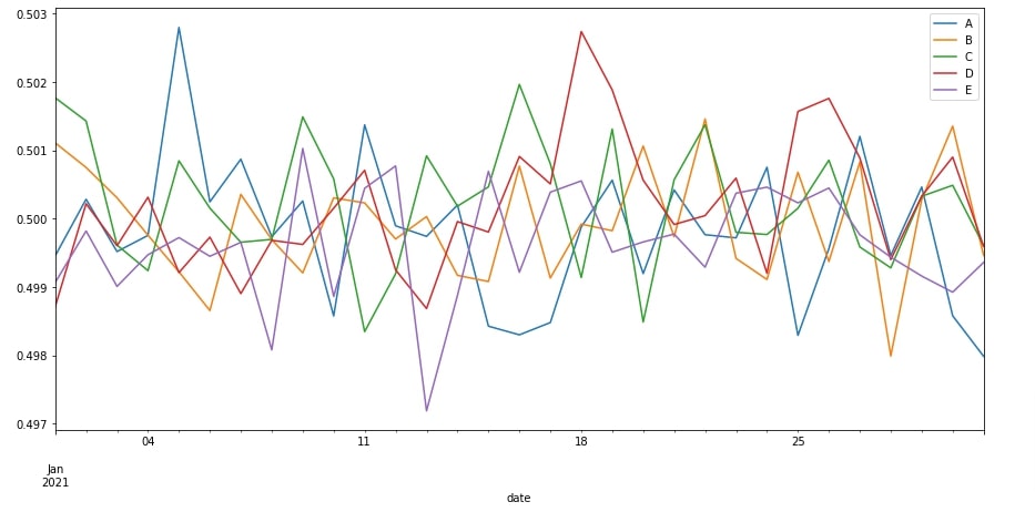
Below we have first resampled our January month dask dataframe at a daily frequency and then taken the average of each day. The final resulting dataframe will have an average of columns for one day of data for each day of January.
We have then simply called plot() method on it which will plot line chart. The line chart will use the index for X-axis and all other columns data for Y-axis.
%matplotlib inline

jan_2021_new.resample("1D").mean().compute().plot(figsize=(15,7));
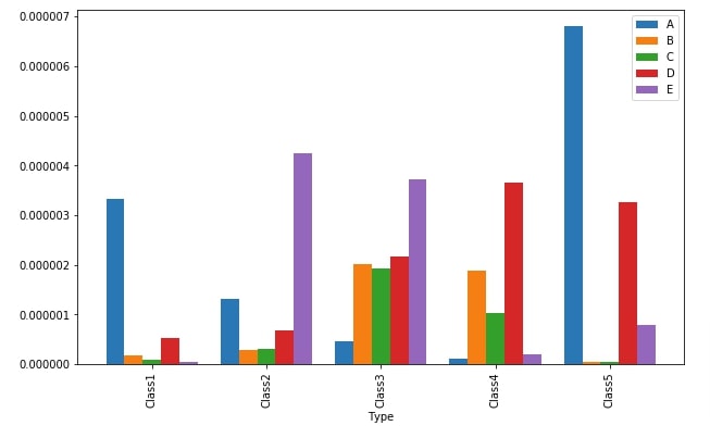
Below we have included another example of plotting. In this example, we have first grouped entries of the January month dataframe according to Type column and calculated the minimum of each column. The resulting dataframe will have a minimum for each column of data for each different value of Type column.
jan_2021_new.groupby(["Type"]).min().compute().plot(kind="bar", width=.8, figsize=(10,6));
 Sunny Solanki
Sunny Solanki
Intro: Software Developer | Youtuber | Bonsai Enthusiast
About: Sunny Solanki holds a bachelor's degree in Information Technology (2006-2010) from L.D. College of Engineering. Post completion of his graduation, he has 8.5+ years of experience (2011-2019) in the IT Industry (TCS). His IT experience involves working on Python & Java Projects with US/Canada banking clients. Since 2020, he’s primarily concentrating on growing CoderzColumn.
His main areas of interest are AI, Machine Learning, Data Visualization, and Concurrent Programming. He has good hands-on with Python and its ecosystem libraries.
Apart from his tech life, he prefers reading biographies and autobiographies. And yes, he spends his leisure time taking care of his plants and a few pre-Bonsai trees.
Contact: sunny.2309@yahoo.in


![YouTube Subscribe]() Comfortable Learning through Video Tutorials?
Comfortable Learning through Video Tutorials?
If you are more comfortable learning through video tutorials then we would recommend that you subscribe to our YouTube channel.
![Need Help]() Stuck Somewhere? Need Help with Coding? Have Doubts About the Topic/Code?
Stuck Somewhere? Need Help with Coding? Have Doubts About the Topic/Code?
 Stuck Somewhere? Need Help with Coding? Have Doubts About the Topic/Code?
When going through coding examples, it's quite common to have doubts and errors.
If you have doubts about some code examples or are stuck somewhere when trying our code, send us an email at coderzcolumn07@gmail.com. We'll help you or point you in the direction where you can find a solution to your problem.
You can even send us a mail if you are trying something new and need guidance regarding coding. We'll try to respond as soon as possible.
![Share Views]() Want to Share Your Views? Have Any Suggestions?
Want to Share Your Views? Have Any Suggestions?
 Want to Share Your Views? Have Any Suggestions?
If you want to
- provide some suggestions on topic
- share your views
- include some details in tutorial
- suggest some new topics on which we should create tutorials/blogs
 dask, dataframes