Dask Array: Guide to Work with Large Arrays in Parallel
Dask is one of the most commonly used parallel computing frameworks of the Python ecosystem. It provides many different sub-modules to perform parallel computing on a single computer or cluster of computers with ease. It let us work with big datasets which do not fit into main memory by dividing datasets and bringing a small part of them into the main memory at the time. It can easily distribute work on the cores of a single computer to multiple computers on the cluster. Below we have listed the most commonly used dask sub-modules designed for various purposes.
- dask.distributed (Futures) - This submodule has the same API as that of concurrent.future module of Python and lets us submit our functions to dask cluster for execution. The code designed using this module works in eager mode compared to all other modules (mentioned below) which work in lazy mode (need to call compute() method to actually start execution). We don't need to call compute() tasks submitted as they will start executing as soon as we submit them to cluster based on the availability of free core/computer/node. If there is no free node then it'll be added to the pending tasks queue and will be executed as soon as free core/computer/node is available for it. The operations are completed immediately returning Future object which will be populated with results when the task is complete. This won't block the normal execution of code.
- dask.bag - This module is designed to work with collection of python objects (lists/iterators) in parallel and perform operations like map(), filter(), groupby(), etc on them. This package is similar to PySpark. This module works in lazy mode hence we need to call compute() method at last to actually perform operations. The execution will wait for completion of task until compute() method returns with results.
- dask.delayed - This module is designed to work with problems when you can't use arrays or dataframes to represent your data. It let us parallelize our existing python functions. This module works in lazy mode hence we need to call compute() method, at last, to actually perform operations. The execution will wait for the completion of the task until compute() method returns with results.
- dask.dataframe - This sub-module let us work on large pandas dataframes in parallel. This module works in lazy mode hence we need to call compute() method, at last, to actually perform operations. The execution will wait for the completion of the task until compute() method returns with results.
- dask.array - This module lets us work on large numpy arrays in parallel. This module works in lazy mode hence we need to call compute() method, at last, to actually perform operations. The execution will wait for the completion of the task until compute() method returns with results.
As a part of this tutorial, we'll be concentrating on dask.array module. We'll explain how we can create arrays and work with them in parallel using dask. The dask.array module implements many functionalities provided by numpy arrays. It implements all functionalities which can be parallelized. Internally dask array itself is composed of many numpy arrays where each array holds part of the main array.

Below we have listed important sections of our tutorial to give an overview of the material covered.
Important Sections of Tutorial
- Create Arrays
- Indexing/Slicing Arrays
- Array Attributes
- Normal Array Operations
- Random Numbers Array
- Simple Statistics
Below we have imported the necessary libraries that we'll use in our tutorial. We have also imported dask.array separately.
import dask

print("Dask Version : {}".format(dask.__version__))
import dask.array as da
import numpy as np
Create Dask Cluster (Optional Step)
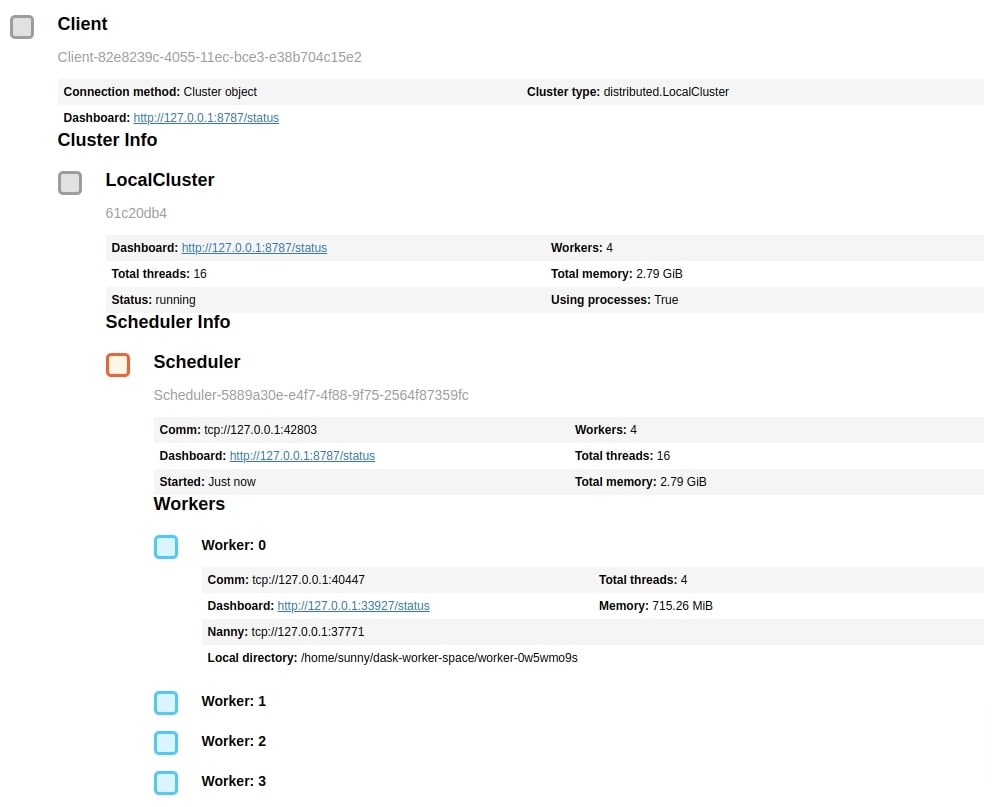
In order to use dask, we'll be creating a cluster of dask workers. This is not a compulsory step as we can continue working with dask arrays without creating dask clusters. But we are creating it to limit memory usage and the number of workers. This cluster also gives us a URL of the dashboard which dask provides to analyze parallel processing it performs behind the scenes. This can help us better understand operations and the time taken by them. The dask cluster we have created below is on a single computer but the dask cluster can be spread across clusters of computers as well.
If you want to know in detail about dask clusters then please feel free to check our below tutorial which explains the architecture of dask along with the cluster creation process.
Below we have created a dask cluster of 4 processes where each process can use 0.75 GB of main memory. We can open the dashboard URL in a separate tab to see the progress of tasks when we execute some tasks on the dask cluster by calling compute() method.
from dask.distributed import Client

client = Client(n_workers=4, threads_per_worker=4, memory_limit='0.75GB')

client
1. Create Arrays 
In this section, we'll explain various ways to create dask arrays. The API of dask.array is almost the same as that of numpy hence the majority of functions will work exactly the same as numpy.
arange()
The arange() method works exactly like python range() function but returns dask array. When creating a dask array by calling this function, it does not actually create an array. It'll only create an array when we call compute() method on it or on any operations performed on it. The dask array are lazy by default just like the majority of dask modules which requires us to call compute() method to actually create and bring data in memory and perform some operations on them.
Below we have created an array using arange() function and displayed it. The below function call completes immediately and does not use any memory as it's just a function call. We have then displayed the array. The jupyter notebook creates a nice representation of the dask array. We can notice that it shows the size of an array, memory usage (when we actually bring it in memory by calling compute()), and data type as well.
It also displays information about chunks. The chunk is a small subset of our original dask array. When we perform any operations on the dask array, it'll bring a single chunk of an array in memory and work on it. At last, it'll combine the results of all chunks to create a final resulting array.
The majority of dask array creation methods accept an argument named 'chunks' which accepts a tuple of integers with the same rank as that of the original array to let dask know about the size of the individual chunks. The integer specifies the number of elements to keep in each dimension of the array. If an array is one dimensional then chunks will have a tuple of size 1, a two-dimensional array will have a tuple of two integers for chunks, and so on. We'll explain through our examples how we can use 'chunks' argument with various methods.
By default, chunks argument is None and dask will create an array with only one chunk. We should divide the dask array into chunks using 'chunks' argument if we want to distribute work across different cores of computer/computers of the cluster for faster computation in parallel. If we keep only one chunk then there won't be parallel computation and operations will be almost like a normal numpy array on a single-core/computer which can be slower for large datasets that can benefit from parallelism.
x = da.arange(100_000)

x
In the next cell, we have created another array using arange() but this time, we have provided chunks argument with tuple (100,). This will keep 100 elements per chunk. As this is a one-dimensional array, we have provided chunk size with a tuple of a single integer. As our main array is of size 100_000, we'll have 1000 chunks which we can easily get by dividing array size by elements per chunk (100,000 / 100 = 1000).
We can notice the representation created of an array this time includes chunk size, shape, and count differently from the previous one chunk array. We can notice the difference in the size of the total array and chunk as well.
x = da.arange(100_000, chunks=(100,))

x
By default, arange() method creates an array of integers but we can ask it to create an array of floats as well by providing dtype argument.
Below we have created a float array using arange() method.
Please make a NOTE that we have provided numpy data type to dtype argument as dask does not have any data type defined in them. Dask is just a wrapper library that performs array operations in parallel on underlying numpy arrays.
x = da.arange(100_000, chunks=(100,), dtype=np.float32)

x
ones()
In the next cell, we have created an array of all 1s using ones() method of dask array. It takes as input shape of an array as the first argument. We have provided chunks as 10 which will use chunk size as 10 in all dimensions. If we provide only a single integer for 'chunks' for a multi-dimensional array then it'll use the same chunk size in all dimensions. In the below example, the chunk size of 10 will be treated as (10,10).
We can notice that our array has total 1_000_000 elements (1000x1000) and single chunk (10x10) is composed of 100 elements (10x10), the total number of chunks will be 10_000 which we can get by dividing total elements by number of elements per chunk (1_000_000 / 100 = 10_000).
x = da.ones((1000,1000), chunks=10, dtype=np.float32)

x
In the next cell, we have again created an array of 1s with dimension 1000x1000 but this time we have given a tuple of two integers to specify chunk size. The tuple (10,100) indicates that 10 elements in first axis and 100 elements in second axis should create one chunk (10 x 100 = 1000 elements per chunk).
x = da.ones((1000,1000), chunks=(10, 100))

x
ones_like()
The ones_like() method takes as input another array and creates an array of 1s with the same dimension as the dimension of the input array.
x = da.arange(100_000, chunks=100)

y = da.ones_like(x)

y
zeros()
The zeros() method works exactly like ones() with only difference that it creates an array of 0s. There is also zeros_like() method which works exactly like ones_like() but creates an array of 0s.
x = da.zeros((10_000,10_000), chunks=(100,100))

x
diag()
The diag() function takes as input another dask array and sets its elements on the diagonal of the square array with all other elements set to 0.
Below we have created a diagonal array where numbers 0-9 are set on diagonal of 2-dimensional array. We have the first time called compute() method on a dask array to retrieve the actual array and display it.
x = da.diag(da.arange(10))

x
x.compute()
empty()
We can create an empty array using the method empty(). The data inside the array generated by this method will be garbage. It accepts the shape of an array as the first argument and should be specified using a tuple. It also accepts chunks argument like other methods.
x = da.empty((100,100), chunks=(10,10))

x.compute()
eye()
The eye() method creates an identity array where all elements on the diagonal will be 1 and all other elements of the array will be 0. It accepts a single integer specifying the size of the array.
x = da.eye(100, chunks=10)

x.compute()
full()
The full() method can create an array whose all elements have the same value. It accepts array shape specified as tuple as the first argument. The second argument should be the element that should be present in an array.
x = da.full((10,10), 12.3)

x.compute()
full_like()
The full_like() method can create an array whose shape can be taken from another array. It takes as input another array and a scalar value.
x = da.zeros((10,5))

y = da.full_like(x, 12.3)

y.compute()
from_array()
We can create a dask array from any existing python list/tuple or numpy array using from_array() method.
Below we have created a dask array from a numpy array of random numbers.
x = np.random.rand(10,10)

y = da.from_array(x)

y
x[0], y[0].compute()
array()
The array() method works exactly like from_array() method and can create a dask array from a python sequence or numpy arrays.
x = np.random.rand(10,10)

y = da.array(x)

y
x[0], y[0].compute()
asarray()
The asarray() is another method which works like methods array() and from_array().
x = np.random.rand(10,10)

y = da.asarray(x)

y
x[0], y[0].compute()
repeat()
The repeat() method takes as input an array and repeats its elements based on the axis to create a new array.
Below we have first created a dask array of five integers from 0-4. We have then called repeat() method asking it to repeat elements 3 times.
x = da.arange(5)

y = da.repeat(x, 3, axis=0)

y.compute()
Below we have first created a dask array of integers in the range 0-6 and then reshaped it as an array of size (2,3).
We have then called repeat() method with our dask array as input and asked it to repeat elements 3 times at axis 1.
We have then called repeat() method again with our dask array as input and asked it to repeat elements 2 times at axis 0.
We have then at last called compute() on both of our new dask arrays to see the results. We can notice from the results that how elements are repeated across different axes.
x = da.arange(6).reshape(2,3)

y = da.repeat(x, 3, axis=1)

z = da.repeat(x, 2, axis=0)

x.compute(), y.compute(), z.compute()
linspace()
The linspace() method can create a dask array by dividing a range into evenly spaced values. We need to provide start and end values of range as well as the number of evenly spaced values to create in that range.
x = da.linspace(1,9,10)

x.compute()
copy()
The copy() method actually creates a copy of the dask array. The new array will be stored at different memory locations hence change in the original array from which it was created, won't affect it.
x = np.random.rand(10,10)

y = da.asarray(x)

z = y.copy()
x[0], y[0].compute(), z[0].compute()
2. Indexing/Slicing Arrays 
In this section, we'll explain with simple examples how we can perform integer indexing/slicing on our dask array. It exactly follows the same rules as that of numpy indexing hence any background with numpy indexing will be useful to follow along this section.
Below we have created an array of random numbers using numpy first. We have then created a dask array from this numpy array using from_array() method. We'll be using this array to explain indexing.
x = np.random.rand(100,100)

arr = da.from_array(x, chunks=(10,10))

arr
Below we have performed integer indexing on our array asking it to take every 5th element from the first dimension and all elements from the second dimension.
As we are taking every 5th element from 100 elements, there will be only 20 elements in our first dimension. We can notice below from array representation that chunk size is also adjusted according to indexing.
arr[::5,:]
Below we have created another example where we are taking every 5th element in both dimensions of our array. This will reduce our 100x100 array to 20x20. The chunk size is also changed from 10x10 to 2x2.
arr[::5, ::5]
arr_part = arr[::5, ::5].compute()

arr_part.shape
3. Array Attributes 
In this section, we'll be explaining the attributes of the dask array.
Below we have created a simple array of integers using arange() method and then reshaped it to shape 100x100.
arr = da.arange(10_000).reshape(100,100)

arr
The shape of the array can be retrieved by calling shape attribute on an array.
arr.shape
The size of an array represents a total number of elements stored in an array and can be retrieved using size attribute.
arr.size
The chunks returns a tuple of the same size as the dimensions of the array. It'll return a tuple of size 1 for a one-dimensional array, the tuple of size 2 for a two-dimensional array, etc. Each individual element of the tuple will be again tuple which will have the number of elements present in the particular chunk of an array.
arr.chunks
The chunksize attribute returns the chunk shape of the dask array.
arr.chunksize
The itemsize attribute returns the number of bytes of memory used by a single element of an array.
arr.itemsize
The nbytes attribute returns the total number of bytes of memory that will be used by this array if we bring it in memory.
arr.nbytes
The dtype represents the type of elements stored in an array.
arr.dtype
We can also name a dask array using name attribute.
arr.name
arr._name = "Array1"

arr.name
The npartitions attribute returns the number of partitions of an array. This attribute returns the number of chunks of an array.
arr.npartitions
Below we have created a two-dimensional array again to explain a few attributes of the dask array again.
arr = da.zeros((100,100), chunks=(10,10))

arr
We can notice here that how chunks attribute returns a tuple of size 2 where both elements are again tuples specifying elements present in the chunk of an array.
arr.chunks
The chunksize is the same as what we provided to chunks argument of the method.
arr.chunksize
arr.npartitions
arr.partitions[0].compute().shape
arr.partitions[0,0].compute().shape
4. Normal Array Operations 
In this section, we'll explain different operations that we can perform on dask array like transpose, dot product, array multiplication, addition, flattening array, changing dimensions, etc. We'll be exploring many methods of dask array in this section.
reshape()
Below we have first created a dask array of 10_000 integers and then reshaped it from one dimension to a two-dimensional array using reshape() method. We have reshaped the array to shape 100x100.
arr = da.arange(10_000).reshape(100,100)

arr
rechunk()
The rechunk() method can be called on any dask array to change the existing chunk size or add chunk size to an array without chunking. It accepts chunk size specified as a tuple or single integer. If a single integer is specified for a multi-dimensional array then the same chunk size will be used in all dimensions.
Below we have re-chunked our array from a single chunk to 100 chunks of size (10,10).
arr.rechunk(chunks=(10,10))
transpose()
The transpose() function can transpose an array.
arr = da.arange(10).reshape(2,5)

arr.transpose()
astype()
The astype() function takes as input a numpy data type and transforms the input array type to the given.
arr.astype(np.float32)
flatten()
The flatten() method flattens multi-dimensional array.
arr.flatten()
dot()
The dot() method calculates the dot product of the current array and another array given as input.
arr.dot(arr.T)
matmul()
The matmul() method is available from dask.array module and can multiply two dask arrays.
da.matmul(arr, arr.T)
Array Addition
We can perform array addition using + operator or add() method available through dask.array module.
arr = da.arange(10).reshape(2,5)

(arr + arr).compute()
da.add(arr, arr).compute()
ravel()
The ravel() method works like flatten() method and flattens dask array.
arr.ravel().compute()
squeeze()
The squeeze() method removes any extra dimension present in the dask array.
Below we have reshaped our array to shape 1x2x5 where the first dimension is extra and can be removed by calling squeeze() method on the array.
x = arr.reshape((1,2,5))

x
x.squeeze()
round()
The round() method will round float elements as its name suggest.
arr = da.random.random((5,2)) * 10

arr.compute(), da.round(arr).compute(), arr.round().compute()
clip()
The clip() method limits the elements of the array in a particular range. It'll replace all elements which fall outside of the specified range with upper and lower limits of the range.
The clip() method is available directly on the dask array as well as from dask.array module.
arr = da.random.random((5,2)) * 10

x = arr.clip(min=0.5, max=5.0)

y = da.clip(arr, 0.5, 5.0)

arr.compute(), x.compute(), y.compute()
all()
The all() method returns True if all elements evaluates to True. If some array elements are 0 then this method will return False.
arr = da.random.random((5,2)) * 10

arr.all().compute()
any()
This method returns True if any element of the dask array evaluates to True. This method will return False if all array elements are 0.
arr = da.random.random((5,2)) * 10

arr.any().compute()
allclose()
The allclose() method available from dask.array module takes as input two dask arrays and returns True if both are equal element-wise else it returns False.
arr1 = da.random.random((5,2)) * 10
arr2 = da.random.random((5,2)) * 10

da.allclose(arr1, arr1).compute(), da.allclose(arr1, arr2).compute()
append()
The append() method available from dask.array module let us append elements to dask array.
arr = da.arange(10)

da.append(arr, [5,10]).compute()
arr = da.arange(10).reshape(2,5)

da.append(arr, arr, axis=0).compute(), da.append(arr, arr, axis=1).compute()
ceil()
The ceil() method returns ceiling values of the input dask array of floats.
arr = da.random.random((5,2)) * 10

da.ceil(arr).compute()
floor()
The floor() method returns floor values of the input dask array of floats.
arr = da.random.random((5,2)) * 10

da.floor(arr).compute()
concatenate()
The concatenate() method available from dask.array module can be used to concatenate more than one array. We can perform concatenation at a particular axis as well. By default, it performs concatenation at the first dimension of the array.
arr1 = da.random.random((5,2)) * 10
arr2 = da.random.random((5,2)) * 10

arr3 = da.concatenate((arr1, arr2))
arr4 = da.concatenate((arr1, arr2), axis=1)

arr3.shape, arr4.shape
isnan() | isnull()
The isnan() or isnull() method available from dask.array module can be used to check presence of NaN / None in dask array. It returns array of same shape as input array with boolean values specifying presence or absence of NaN / None.
arr1 = da.random.random((5,2)) * 10

arr1[1,0] = np.nan
arr1[2,1] = np.nan
arr1[3,1] = np.nan

da.isnan(arr1).compute(), da.isnull(arr1).compute()
where()
The where() method available from dask.array module can let us make conditional decisions on an array. The array elements are selected based on condition. The first argument is a condition, the second argument is value to use when the condition evaluates to True and the third argument is value to use when the condition evaluates to False.
Below we have first created a dask of random numbers with the shape of (5,2). We have then checked for the condition of elements greater than 5 using method where(). We return an array of the same shape as the input array where elements greater than 5 will be True and elements less than that will be False.
arr1 = da.random.random((5,2)) * 10

x = da.where(arr1 > 5., True, False)

arr1.compute(), x.compute()
Below we have created another example where we are checking for the condition greater than 5 again with where() method. This time we have provided the second and third argument dask array of the same shape as the input array. The array provided for cases when the condition evaluates to True is an array of 1s and the array provided for cases when the condition evaluates to False is an array of 0s.
arr1 = da.random.random((5,2)) * 10
arr2 = da.ones_like(arr1)
arr3 = da.zeros_like(arr1)

x = da.where(arr1 > 5., arr2, arr3)

arr1.compute(), x.compute()
unique()
The unique() method available from dask.array takes as input dask array and removes duplicate elements from the array.
arr = da.array([1,2,1,3,4,5,1,2])

da.unique(arr).compute()
pad()
The pad() function available from dask.array module can be used to add padding of specified size around the array. It takes as input dask array and padding size specified as single integer or tuple of integers.
arr = da.random.random((3,2))

x = da.pad(arr, 2)

x.compute()
hstack() | vstack()
The hstack() and vstack() methods are used to horizontally and vertically merge input arrays.
Below we have explained the usage of both methods with simple and easy-to-understand examples.
arr1 = da.arange(10).reshape(5,2)
arr2 = da.arange(10,20).reshape(5,2)

x = da.vstack((arr1, arr2))
y = da.hstack((arr1, arr2))

arr1.compute(), arr2.compute(), x.compute(), y.compute()
stack()
The stack() method can be used to merge input arrays at a particular axis.
Below we have explained its usage with a simple example. Please take a look at how arrays are merged at a particular axis and compare it with an output of methods hstack() and vstack() from the previous cell. The stack() method creates one extra dimension when merging arrays.
arr1 = da.arange(10).reshape(5,2)
arr2 = da.arange(10,20).reshape(5,2)

x = da.stack((arr1,arr2), axis=0)

y = da.stack((arr1,arr2), axis=1)

x = x.compute()
y = y.compute()

print(x.shape, y.shape)

x, y
absolute()
The absolute() method available from dask.array module returns an array where values of input array are replaced with absolute values.
arr1 = da.random.random((5,2)) * 10

arr1[0,0] = -1.5
arr1[1,1] = -2.5

da.absolute(arr1).compute()
Few other Methods
Below we have listed a few other methods available from dask.array module that can be used for various purposes.
da.log, da.log2, da.exp, da.sin, da.sinh, da.tan, da.tanh, da.cos, da.cosh, da.power, da.floor
5. Random Numbers Array 
In this section, we'll explain various methods available through dask.array.random module to create dask arrays of random numbers.
random()
This method takes shape of an array specified as tuple and chunk size specified as integer/tuple as input and creates a dask array of random numbers in the range 0-1.
arr = da.random.random(size=(5,5), chunks=(2,2))

arr
arr.compute()
randint()
The randint() method lets us create a dask array of random integers in the specified range. We can specify the range as the first two values of the method followed by array shape specified as a tuple of integers. We can also provide chunk size with chunks parameter.
arr = da.random.randint(1,100,size=(5,5), chunks=(2,2))

arr.compute()
choice()
The choice() method creates an array of numbers randomly selected from the input array. It takes another 1D array of numbers and the shape of an array as input and creates an array by randomly selecting elements from the input array.
arr = da.arange(100)

x = da.random.choice(arr, size=(5,5), chunks=(2,2))

x.compute()
normal()
This method lets us create a dask array of random numbers selected from normal (gaussian) distribution. It takes the mean of the distribution as the first parameter and standard deviation as the second parameter followed by the array shape specified as a tuple. It then creates normal distribution and draws numbers randomly from it.
arr = da.random.normal(loc=0, scale=2, size=(5,5), chunks=(2,2))

arr.compute()
uniform()
This method creates a dask array of random numbers selected from a uniform distribution. It takes a lower limit of distribution as the first parameter and a higher limit of distribution as the second parameter followed by an array shape specified as a tuple. It then creates uniform distribution and draws numbers randomly from it.
arr  = da.random.uniform(low=0.0, high=2.0, size=(5,5), chunks=(2,2))

arr.compute()
binomial()
This method creates a dask array of random numbers drawn from a binomial distribution. The first two parameters are input parameters for binomial distribution followed by the shape of the array specified as a tuple. The first parameter is a number of experiments and should be integer >=0. The second parameter is probability and should float in the range (0,1).
arr = da.random.binomial(2,0.5, size=(5,5), chunks=(2,2))

arr.compute()
multinomial()
This method creates a dask array of random numbers drawn from a multinomial distribution. The first two parameters are input parameters for multinomial distribution followed by the shape of the array specified as a tuple. The first parameter is a number of experiments and should be integer >=0. The second parameter is a list of p-values (specified as floats in the range 0-1) for different outcomes of experiments. The sum of all p-values should be 1. The method creates multinomial distribution using parameters and draws numbers randomly from it to create an array.
arr = da.random.multinomial(2, [1/4,]*4, size=(5,5), chunks=(2,2))

arr.compute()
chisquare()
This method creates a dask array of random numbers drawn from the chi-squared distribution. This method accepts one parameter for distribution creation followed by an array shape specified as a tuple of integers. The first parameter is a degree of freedom of chi-squared distribution and should be integer >0. The method creates chi-squared distribution from it and draws numbers randomly from it.
arr = da.random.chisquare(2, size=(5,5), chunks=(2,2))

arr.compute()
poisson()
This method creates a dask array of random numbers drawn from the Poisson distribution. This method accepts one parameter for distribution creation followed by an array shape specified as a tuple of integers. The first parameter is the expectation of interval of Poisson distribution and should be float value >=0. The method creates Poisson distribution from it and draws numbers randomly from it.
arr = da.random.poisson(lam=1.,size=(5,5), chunks=(2,2))

arr.compute()
6. Simple Statistics 
In this section, we'll explain various methods available through dask.array to perform various statistical operations like min, max, mean, median, cumulative sum, cumulative product, etc.
Below we have created a dask array of random numbers of shape 3x5. We'll be using this array to explain various statistical operations available through dask.array.
arr = da.random.random(size=(3,5), chunks=(2,2))

arr
arr.compute()
min() | max()
The min() function returns minimum element of the dask array and max() function returns maximum element of dask array.
We can also provide axis details to both methods to retrieve minimums/maximums at a particular axis of our dask array.
arr.min().compute()
arr.max().compute()
arr.min(axis=0).compute(), arr.min(axis=1).compute(),
arr.max(axis=0).compute(), arr.max(axis=1).compute(),
argmin() | argmax()
The argmin() and argmax() methods works like min() and max() methods but returns index of minimum and maximum elements.
arr.argmin(axis=0).compute(), arr.argmin(axis=1).compute(),
arr.argmax(axis=0).compute(), arr.argmax(axis=1).compute(),
sum()
The sum() method returns the sum of all values of the dask array. We can retrieve the sum at a particular axis of an array as well using axis argument.
arr.sum().compute()
arr.sum(axis=0).compute(), arr.sum(axis=1).compute()
mean()
The mean() method returns an average of array elements. We can retrieve the mean at a particular axis of the dask array using axis argument.
arr.mean().compute()
arr.mean(axis=0).compute(), arr.mean(axis=1).compute()
std()
The std() method returns standard deviation of array elements. We can retrieve standard deviation at a particular axis of the dask array using axis argument.
arr.std().compute()
arr.std(axis=0).compute(), arr.std(axis=1).compute()
cumsum()
The cumsum() method cumulative sum of array elements. We can retrieve the cumulative sum at a particular axis of the dask array using axis argument.
arr.cumsum(axis=0).compute()
arr.cumsum(axis=1).compute()
cumprod()
The cumprod() method returns cumulative product of array elements. We can retrieve cumulative product at the particular axis of the dask array using axis argument.
arr.cumprod(axis=0).compute()
arr.cumprod(axis=1).compute()
var()
The var() method returns variance of array elements. We can retrieve variance at a particular axis of the dask array using axis argument.
arr.var().compute()
arr.var(axis=0).compute(), arr.var(axis=1).compute()
corrcoef()
We can calculate correlation between two dask arrays using corrcoef() method.
arr1 = da.linspace(1,10,5)
arr2 = da.linspace(1,20,5)

arr1.compute(), arr2.compute()
da.corrcoef(arr1, arr2).compute()
maximum()
The maximum() method takes two dask arrays as input and returns an array that has the same length as input arrays but elements are element-wise maximum.
arr1 = da.linspace(1,10,5)
arr2 = da.random.random(5) *5

arr1.compute(), arr2.compute()
da.maximum(arr1, arr2).compute()
This ends our small tutorial explaining how we can use dask.array module to create, index/slice, manipulate and calculate simple statistics on dask arrays. Please feel free to let us know your views in the comments section.
References
 Sunny Solanki
Sunny Solanki
Intro: Software Developer | Youtuber | Bonsai Enthusiast
About: Sunny Solanki holds a bachelor's degree in Information Technology (2006-2010) from L.D. College of Engineering. Post completion of his graduation, he has 8.5+ years of experience (2011-2019) in the IT Industry (TCS). His IT experience involves working on Python & Java Projects with US/Canada banking clients. Since 2020, he’s primarily concentrating on growing CoderzColumn.
His main areas of interest are AI, Machine Learning, Data Visualization, and Concurrent Programming. He has good hands-on with Python and its ecosystem libraries.
Apart from his tech life, he prefers reading biographies and autobiographies. And yes, he spends his leisure time taking care of his plants and a few pre-Bonsai trees.
Contact: sunny.2309@yahoo.in


![YouTube Subscribe]() Comfortable Learning through Video Tutorials?
Comfortable Learning through Video Tutorials?
If you are more comfortable learning through video tutorials then we would recommend that you subscribe to our YouTube channel.
![Need Help]() Stuck Somewhere? Need Help with Coding? Have Doubts About the Topic/Code?
Stuck Somewhere? Need Help with Coding? Have Doubts About the Topic/Code?
 Stuck Somewhere? Need Help with Coding? Have Doubts About the Topic/Code?
When going through coding examples, it's quite common to have doubts and errors.
If you have doubts about some code examples or are stuck somewhere when trying our code, send us an email at coderzcolumn07@gmail.com. We'll help you or point you in the direction where you can find a solution to your problem.
You can even send us a mail if you are trying something new and need guidance regarding coding. We'll try to respond as soon as possible.
![Share Views]() Want to Share Your Views? Have Any Suggestions?
Want to Share Your Views? Have Any Suggestions?
 Want to Share Your Views? Have Any Suggestions?
If you want to
- provide some suggestions on topic
- share your views
- include some details in tutorial
- suggest some new topics on which we should create tutorials/blogs
 dask-array, parallel-computing, distributed-computing