Scikit-Learn - Naive Bayes for Classification Tasks
Naive Bayes estimators are probabilistic estimators based on the Bayes theorem with the naive assumption that there is conditional independence between features of data.
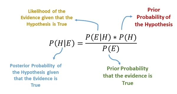
> Bayes Theorem
The Bayes Theorem helps us determine the probability of occurring events based on prior knowledge of conditions that can be related to the event.
The naive Bayes classifiers have worked quite well for document classification and spam filtering applications.
It requires a small amount of training data to set up probabilities for Bayes theorem and therefore works quite fast.
Due to their simplicity, they are quite fast compared to many ML algorithms.
> What Can You Learn From This Article?
As a part of this tutorial, we have explained how to use naive Bayes classifiers / estimators available from Python library scikit-learn for classification tasks with simple and easy-to-understand examples. Tutorial uses a digits dataset for explaining each estimator. We fit train data to naive Bayes models, evaluate their performance on test data and also perform hyperparameters tuning to further improve performance.
Below, we have listed important sections of tutorial to give an overview of the material covered.
Important Sections Of Tutorial
- Naive Bayes Estimators from Scikit-Learn
- Load Digits Dataset
- Split Dataset into Train & Test Sets
- Visualize Few Data Examples
- BernoulliNB
- Train Model
- Evaluate Model
- Calculate Accuracy Score & Classification Report
- Visualize Confusion Matrix
- Hyperparameters Tuning using Grid Search
- Evaluate Performance Of Fine Tuned Model
- Calculate Accuracy Score & Classification Report
- Visualize Confusion Matrix
- Evaluate Performance Of Fine Tuned Model
- GaussianNB
- ComplementNB
- MultinomialNB
- CategoricalNB
- Summary Of Results
- Naive Bayes for Large Datasets
We'll start by importing the necessary Python libraries for our tutorial.
import numpy as np
import pandas as pd
import matplotlib.pyplot as plt

import sklearn

print("Scikit-Learn Version : {}".format(sklearn.__version__))

np.set_printoptions(precision=2)

%matplotlib inline
Below, we have listed different types of naive Bayes estimators available from scikit-learn.
1. Naive Bayes Estimators from Scikit-Learn 
Scikit-Learn provides a list of 5 Naive Bayes estimators where each differs from other based on probability of particular feature appearing if particular class appears:
- BernoulliNB - It represents a classifier that is based on data that is multivariate Bernoulli distributions.
- The Bernoulli distribution implies that data can have multiple features but each one is assumed to be a binary variable.
- GaussianNB - It represents a classifier that is based on the assumption that likelihood of features is Gaussian distribution.
- ComplementNB - It represents a classifier that uses a complement of each class to compute model weights.
- It's a standard variant of multinomial naive Bayes which is well suited for imbalanced class classification problems.
- MultinomialNB - It represents a classifier suited for multinomially distributed data.
- It is well suited for text classification tasks.
- CategoricalNB - It represents a classifier that is best suited for categorically distributed data.
- The datasets that have categorical features are good candidates for working with this estimator.
We'll be explaining the usage of each one of the naive Bayes variants with examples.
2. Load Digits Dataset 
We'll be using digits dataset for our explanation purpose. It has data about every 0-9 digits as an 8x8 pixel image. Each sample image is kept as a vector of size 64.
from sklearn.datasets import load_boston, load_digits

digits = load_digits()

X_digits, Y_digits = digits.data, digits.target

print('Dataset Size : ', X_digits.shape, Y_digits.shape)
n_features, n_classes = X_digits.shape[1], np.unique(Y_digits)

n_features, n_classes
2.1 Splitting Data Into Train/Test Sets
We'll split the dataset into two parts:
- Training data will be used for the training model.
- Test data against which accuracy of the trained model will be checked.
The train_test_split() function of model_selection module of sklearn will help us split data into two sets with 80% for training and 20% for test purposes. We are also using seed(random_state=123) with train_test_split so that we always get the same split and can reproduce results in the future as well.
Please make a note that we are also using stratify parameter which will prevent unequal distribution of all classes in train and test sets.For each class, we'll have 80% samples in train set and 20% samples in test set. This will make sure that we don't have any dominating class in either train or test set.
from sklearn.model_selection import train_test_split

X_train, X_test, Y_train, Y_test = train_test_split(X_digits, Y_digits, train_size=0.80,
                                                    test_size=0.20, stratify=Y_digits, random_state=123)

print('Train/Test Sizes : ', X_train.shape, X_test.shape, Y_train.shape, Y_test.shape)
X_digits.min(), X_digits.max()
2.2 Visualize Few Data Examples
Below, we have visualized few images from dataset using matplotlib.
fig = plt.figure(figsize=(12,5))
plt.imshow(np.hstack(X_digits[:10].reshape(10,8,8)), cmap="gray");
plt.xticks([], []);
plt.yticks([], []);

3. BernoulliNB 
The first estimator that we'll be introducing is BernoulliNB available with the naive_bayes module of sklearn. We'll first fit it with default parameters to data and then will try to improve its performance by doing hyperparameter tuning. We'll also evaluate its performance using a confusion matrix. We'll even inform you regarding important attributes of BernoulliNB which can give helpful insight once the model is trained.
3.1 Train Model (with Default Parameters)
We'll be fitting model to train data by using fit() method of estimator passing it train features and train labels. We are fitting a default model to train data without setting any parameter explicitly.
from sklearn.naive_bayes import BernoulliNB

bernoulli_nb =  BernoulliNB()
bernoulli_nb.fit(X_train, Y_train)
3.2 Evaluate Model Performance
Almost all models in Scikit-Learn API provide predict() method which can be used to predict target values on Test Set passed to it.
Y_preds = bernoulli_nb.predict(X_test)

print(Y_preds[:15])
print(Y_test[:15])

print('\nTest Accuracy : {:.3f}'.format(bernoulli_nb.score(X_test, Y_test))) ## Score method also evaluates accuracy for classification models.
print('Training Accuracy : {:.3f}'.format(bernoulli_nb.score(X_train, Y_train)))
Below, we have calculated classification report for our test predictions. The classification report has precision, recall and f1-score ML metrics for each target class. This can help us understand our model performance for each individual target class.
We have used functions available from 'metrics' sub-module of scikit-learn to calculate ML metrics. Scikit-learn provides many metrics for ML tasks. Please feel free to check below link to know about various ML metrics. It covers majority of them.
from sklearn.metrics import classification_report, accuracy_score

print("Accuracy Score : {:.3f}".format(accuracy_score(Y_test, Y_preds)))
print("\nClassification Report :")
print(classification_report(Y_test, Y_preds))
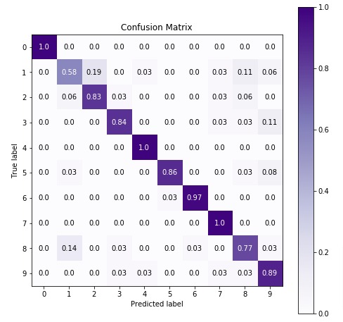
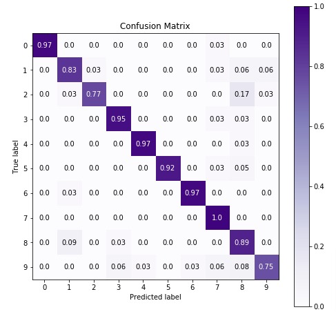
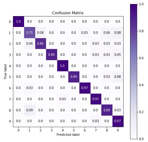
We'll be plotting the confusion matrix to better understand the performance of our model. We have used Python library scikit-plot to visualize confusion matrix. We just need to provide actual labels and predicted labels to method.
Please feel free to check below link if you want to learn about various ML metric visualizations available from scikit-plot. The tutorial covers the whole library with simple examples.
import scikitplot as skplt

fig = plt.figure(figsize=(8,8))
ax = fig.add_subplot(111)
skplt.metrics.plot_confusion_matrix(Y_test, Y_preds,
                                    normalize=True,
                                    title="Confusion Matrix",
                                    cmap="Purples",
                                    ax=ax
                                    );
3.3 Important Attributes of "BernoulliNB"
Below is a list of important attributes available through estimator instance of BernoulliNB.
class_log_prior_- It represents log probability of each class.feature_log_prob_- It represents log probability of a particular feature based on class. (n_classes x n_features)
bernoulli_nb.class_log_prior_
print("Log Probability of Each Feature per class : ", bernoulli_nb.feature_log_prob_.shape)
3.4 Hyperparameters Tuning using Grid Search
Below is a list of common hyperparameters that needs tuning for getting best fit for our data. We'll try various hyperparameters settings to various splits of train/test data to find out best fit which will have almost the same accuracy for both train & test datasets or have quite less difference between accuracy.
> Parameters to Tune
- alpha - It accepts float values representing the additive smoothing parameter. The value of 0.0 represents no smoothing. The default value of this parameter is 1.0.
- fit_prior - It accepts boolean value specifying whether to learn prior class probabilities or not.
- class_prior - It accepts arrays of shape (n_classes,) specifying prior probabilities of target classes.
- binarize - It accepts float value specifying threshold for binarizing data features. The default is None and features are already considered binarized.
Scikit learn provides a class named GridSearchCV that can be used to perform hyperparameters tuning.
GridSearchCV is a wrapper class provided by sklearn which loops through all parameters provided as params_grid parameter with a number of cross-validation folds provided as cv parameter, evaluates model performance on all combinations, and stores all results in cvresults attribute. It also stores model which performs best in all cross-validation folds in bestestimator attribute and best score in bestscore attribute.
If you are someone who is new to hyperparameters tuning using grid search then we would recommend you to check below link. It covers topic in detail.
n_jobs parameter is provided by many estimators. It accepts the number of cores to use for parallelization. If value of -1 is given then it uses all cores. It uses joblib parallel processing library for running things in parallel in background.
We'll below try various values for the above-mentioned hyperparameters to find the best estimator for our dataset by splitting data into 5-fold cross-validation.
%%time

from sklearn.model_selection import GridSearchCV

params = {'alpha': [0.01, 0.1, 0.5, 1.0, 10.0],
          'fit_prior': [True, False],
          'class_prior': [None, [0.1,]* len(n_classes), ],
          'binarize': [None, 0.0, 8.5, 10.0]
         }

bernoulli_nb_grid = GridSearchCV(BernoulliNB(), param_grid=params, n_jobs=-1, cv=5, verbose=5)
bernoulli_nb_grid.fit(X_train,Y_train)

print('Best Parameters : {}'.format(bernoulli_nb_grid.best_params_))
print('Best Accuracy Through Grid Search : {:.3f}\n'.format(bernoulli_nb_grid.best_score_))
3.4.1 Evaluate Performance Of Fine Tuned Model
Below, we have calculated accuracy and classification report on predictions made using best estimators we found through grid search. We can notice a slight improvement in model performance.
from sklearn.metrics import classification_report, accuracy_score

Y_preds = bernoulli_nb_grid.best_estimator_.predict(X_test)
Y_preds_train = bernoulli_nb_grid.best_estimator_.predict(X_train)

print("Test Accuracy Score : {:.3f}".format(accuracy_score(Y_test, Y_preds)))
print("Train Accuracy Score : {:.3f}".format(accuracy_score(Y_train, Y_preds_train)))
print("\nClassification Report :")
print(classification_report(Y_test, Y_preds))
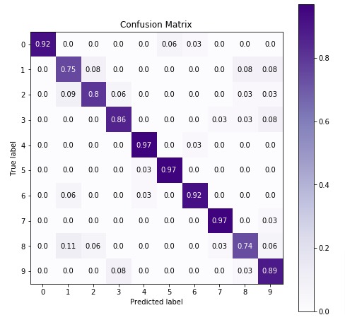
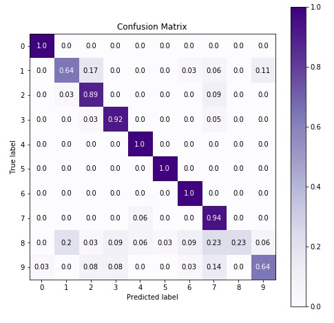
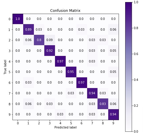
Below we are plotting the confusion matrix again with the best estimator that we found using grid search.
import scikitplot as skplt

fig = plt.figure(figsize=(8,8))
ax = fig.add_subplot(111)
skplt.metrics.plot_confusion_matrix(Y_test, Y_preds,
                                    normalize=True,
                                    title="Confusion Matrix",
                                    cmap="Purples",
                                    ax=ax
                                    );
4. GaussianNB 
The first estimator that we'll be introducing is GaussianNB available with the naive_bayes module of sklearn. We'll first fit it with default parameters to data and then will try to improve its performance by doing hyperparameter tuning. We'll also evaluate its performance using a confusion matrix. We'll even inform you regarding important attributes of GaussianNB which can give helpful insight once the model is trained.
4.1 Train Model (with Default Parameters)
from sklearn.naive_bayes import GaussianNB

gaussian_nb = GaussianNB()
gaussian_nb.fit(X_train, Y_train)
4.2 Evaluate Model Performance
Below, we have made predictions on test dataset using our trained model and then calculated accuracy of test & train predictions.
Y_preds = gaussian_nb.predict(X_test)

print(Y_preds[:15])
print(Y_test[:15])

print('\nTest Accuracy : {:.3f}'.format(gaussian_nb.score(X_test, Y_test))) ## Score method also evaluates accuracy for classification models.
print('Training Accuracy : {:.3f}'.format(gaussian_nb.score(X_train, Y_train)))
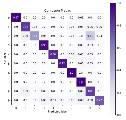
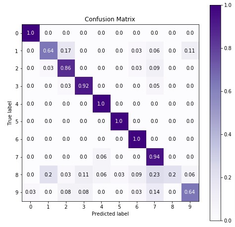
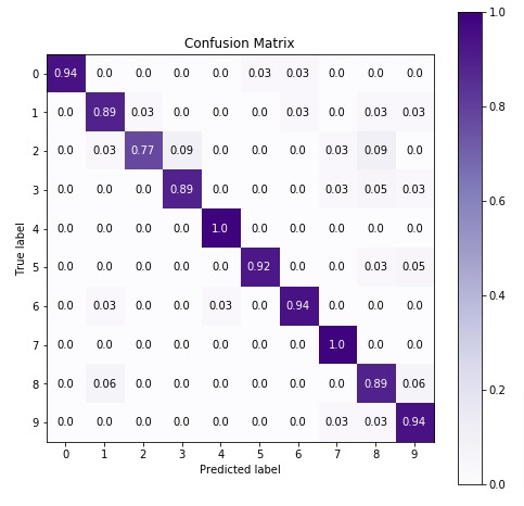
Below, we have calculated accuracy score and classification report on test predictions for evaluation purposes.
In the next cell, we have visualized confusion matrix on test predictions.
from sklearn.metrics import classification_report, accuracy_score

print("Accuracy Score : {:.3f}".format(accuracy_score(Y_test, Y_preds)))
print("\nClassification Report :")
print(classification_report(Y_test, Y_preds))
import scikitplot as skplt

fig = plt.figure(figsize=(8,8))
ax = fig.add_subplot(111)
skplt.metrics.plot_confusion_matrix(Y_test, Y_preds,
                                    normalize=True,
                                    title="Confusion Matrix",
                                    cmap="Purples",
                                    ax=ax
                                    );
4.3 Important Attributes of "GaussianNB"
Below are list of important attributes available through estimator instance of GaussianNB.
class_log_prior_- It represents log probability of each class.epsilon_- It represents absolute additive value to variances.var_- It represents variance of each feature per class. (n_classes x n_features)theta_- It represents mean of feature per class. (n_classes x n_features)
gaussian_nb.class_prior_
gaussian_nb.epsilon_
print("Gaussian Naive Bayes Sigma Shape : {}".format(gaussian_nb.var_.shape))
print("Gaussian Naive Bayes Theta Shape : {}".format(gaussian_nb.theta_.shape))
4.4 Hyperparameters Tuning using Grid Search
Below is a list of common hyperparameters that needs tuning for getting best fit for our data. We'll try various hyperparameters settings to various splits of train/test data to find out best fit which will have almost the same accuracy for both train & test datasets or have quite less difference between accuracy.
> Parameters to Tune
- priors - It accepts arrays of shape (n_classes,) specifying prior probabilities of target classes.
- var_smoothing - It accepts float specifying portion of largest variance of all features that is added to variances for smoothing.
We'll below try various values for the above-mentioned hyperparameters to find the best estimator for our dataset by splitting data into 5-fold cross-validation.
%%time

params = {
            'priors': [None, [0.1,]* len(n_classes),],
            'var_smoothing': [1e-9, 1e-6, 1e-12],
         }

gaussian_nb_grid = GridSearchCV(GaussianNB(), param_grid=params, n_jobs=-1, cv=5, verbose=5)
gaussian_nb_grid.fit(X_train,Y_train)

print('Best Accuracy Through Grid Search : {:.3f}'.format(gaussian_nb_grid.best_score_))
print('Best Parameters : {}\n'.format(gaussian_nb_grid.best_params_))
4.4.1 Evaluate Performance Of Fine Tuned Model
Below, we have calculated accuracy and classification report on predictions made using best estimators we found through grid search. We can notice a slight improvement in model performance.
from sklearn.metrics import classification_report, accuracy_score

Y_preds = gaussian_nb_grid.best_estimator_.predict(X_test)
Y_preds_train = gaussian_nb_grid.best_estimator_.predict(X_train)

print("Test Accuracy Score : {:.3f}".format(accuracy_score(Y_test, Y_preds)))
print("Train Accuracy Score : {:.3f}".format(accuracy_score(Y_train, Y_preds_train)))
print("\nClassification Report :")
print(classification_report(Y_test, Y_preds))
Below we are plotting confusion matrix again with best estimator that we found using grid search.
import scikitplot as skplt

fig = plt.figure(figsize=(8,8))
ax = fig.add_subplot(111)
skplt.metrics.plot_confusion_matrix(Y_test, Y_preds,
                                    normalize=True,
                                    title="Confusion Matrix",
                                    cmap="Purples",
                                    ax=ax
                                    );
5. ComplementNB 
The first estimator that we'll be introducing is ComplementNB available with the naive_bayes module of sklearn. We'll first fit it with default parameters to data and then will try to improve its performance by doing hyperparameter tuning. We'll also evaluate its performance using a confusion matrix. We'll even inform you regarding important attributes of ComplementNB which can give helpful insight once the model is trained.
5.1 Train Model (with Default Parameters)
from sklearn.naive_bayes import ComplementNB

complement_nb = ComplementNB()
complement_nb.fit(X_train, Y_train)
5.2 Evaluate Model Performance
Below, we have made prediction on test dataset using our trained model and then calculated accuracy of test & train predictions.
Y_preds = complement_nb.predict(X_test)

print(Y_preds[:15])
print(Y_test[:15])

print('Test Accuracy : {:.3f}'.format(complement_nb.score(X_test, Y_test))) ## Score method also evaluates accuracy for classification models.
print('Training Accuracy : {:.3f}'.format(complement_nb.score(X_train, Y_train)))
Below, we have calculated accuracy score and classification report on test predictions for evaluation purposes.
In the next cell, we have visualized confusion matrix on test predictions.
from sklearn.metrics import classification_report, accuracy_score

print("Accuracy Score : {:.3f}".format(accuracy_score(Y_test, Y_preds)))
print("\nClassification Report :")
print(classification_report(Y_test, Y_preds))
import scikitplot as skplt

fig = plt.figure(figsize=(8,8))
ax = fig.add_subplot(111)
skplt.metrics.plot_confusion_matrix(Y_test, Y_preds,
                                    normalize=True,
                                    title="Confusion Matrix",
                                    cmap="Purples",
                                    ax=ax
                                    );
5.3 Important Attributes of ComplementNB
Below are list of important attributes available through estimator instance of ComplementNB.
class_log_prior_- It represents log probability of each class.feature_log_prob_- It represents log probability of particular feature based on class. (n_classes x n_features)
complement_nb.class_log_prior_
print("Log Probability of Each Feature per class : {}".format(complement_nb.feature_log_prob_.shape))
5.4 Fine Tuning Model By Doing Grid Search On Various Hyperparameters
Below is a list of common hyperparameters that needs tuning for getting best fit for our data. We'll try various hyperparameters settings to various splits of train/test data to find out best fit which will have almost the same accuracy for both train & test datasets or have quite less difference between accuracy.
> Parameters to Tune
- alpha - It accepts float values representing the additive smoothing parameter. The value of 0.0 represents no smoothing. The default value of this parameter is 1.0.
- fit_prior - It accepts boolean value specifying whether to learn prior class probabilities or not.
- norm - It accepts a boolean value specifying whether to perform second normalization of weights or not.
- class_prior - It accepts arrays of shape (n_classes,) specifying prior probabilities of target classes.
We'll below try various values for the above-mentioned hyperparameters to find the best estimator for our dataset by splitting data into 5-fold cross-validation.
%%time

params = {'alpha': [0.01, 0.1, 0.5, 1.0, 10.0, ],
          'fit_prior': [True, False],
          'norm': [True, False],
          'class_prior': [None, [0.1,]* len(n_classes), ]
         }

complement_nb_grid = GridSearchCV(ComplementNB(), param_grid=params, n_jobs=-1, cv=5, verbose=5)
complement_nb_grid.fit(X_train,Y_train)

print('Best Accuracy Through Grid Search : {:.3f}'.format(complement_nb_grid.best_score_))
print('Best Parameters : {}\n'.format(complement_nb_grid.best_params_))
5.4.1 Evaluate Performance Of Fine Tuned Model
Below, we have calculated accuracy and classification report on predictions made using best estimators we found through grid search. We can notice a slight improvement in model performance.
from sklearn.metrics import classification_report, accuracy_score

Y_preds = complement_nb_grid.best_estimator_.predict(X_test)
Y_preds_train = complement_nb_grid.best_estimator_.predict(X_train)

print("Test Accuracy Score : {:.3f}".format(accuracy_score(Y_test, Y_preds)))
print("Train Accuracy Score : {:.3f}".format(accuracy_score(Y_train, Y_preds_train)))
print("\nClassification Report :")
print(classification_report(Y_test, Y_preds))
Below we are plotting confusion matrix again with best estimator that we found using grid search.
import scikitplot as skplt

fig = plt.figure(figsize=(8,8))
ax = fig.add_subplot(111)
skplt.metrics.plot_confusion_matrix(Y_test, Y_preds,
                                    normalize=True,
                                    title="Confusion Matrix",
                                    cmap="Purples",
                                    ax=ax
                                    );
6. MultinomialNB 
The first estimator that we'll be introducing is MultinomialNB available with the naive_bayes module of sklearn. We'll first fit it with default parameters to data and then will try to improve its performance by doing hyperparameter tuning. We'll also evaluate its performance using a confusion matrix. We'll even inform you regarding important attributes of MultinomialNB which can give helpful insight once the model is trained.
6.1 Train Model (with Default Parameters)
from sklearn.naive_bayes import MultinomialNB

multinomial_nb = MultinomialNB()
multinomial_nb.fit(X_train, Y_train)
6.2 Evaluate Model Performance
Below, we have made prediction on test dataset using our trained model and then calculated accuracy of test & train predictions.
Y_preds = multinomial_nb.predict(X_test)

print(Y_preds[:15])
print(Y_test[:15])

print('\nTest Accuracy : {:.3f}'.format(multinomial_nb.score(X_test, Y_test))) ## Score method also evaluates accuracy for classification models.
print('Training Accuracy : {:.3f}'.format(multinomial_nb.score(X_train, Y_train)))
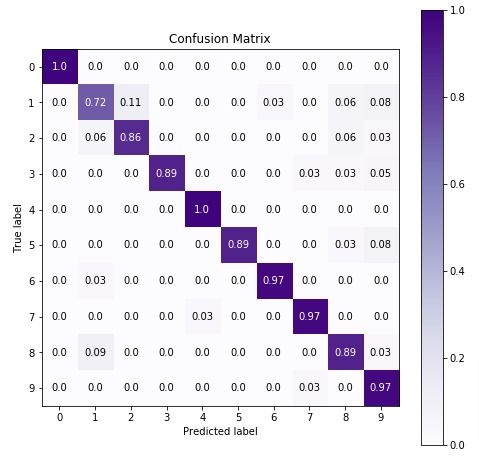
Below, we have calculated accuracy score and classification report on test predictions for evaluation purposes.
In the next cell, we have visualized confusion matrix on test predictions.
from sklearn.metrics import classification_report, accuracy_score

print("Accuracy Score : {:.3f}".format(accuracy_score(Y_test, Y_preds)))
print("\nClassification Report :")
print(classification_report(Y_test, Y_preds))
import scikitplot as skplt

fig = plt.figure(figsize=(8,8))
ax = fig.add_subplot(111)
skplt.metrics.plot_confusion_matrix(Y_test, Y_preds,
                                    normalize=True,
                                    title="Confusion Matrix",
                                    cmap="Purples",
                                    ax=ax
                                    );
6.3 Important Attributes of MultinomialNB
Below are list of important attributes available through estimator instance of MultinomialNB.
class_log_prior_- It represents log probability of each class.feature_log_prob_- It represents log probability of particular feature based on class. (n_classes x n_features)
multinomial_nb.class_log_prior_
print("Log Probability of Each Feature per class : {}".format(multinomial_nb.feature_log_prob_.shape))
6.4 Fine Tuning Model By Doing Grid Search On Various Hyperparameters.
Below is a list of common hyperparameters that needs tuning for getting best fit for our data. We'll try various hyperparameters settings to various splits of train/test data to find out best fit which will have almost the same accuracy for both train & test datasets or have quite less difference between accuracy.
> Parameters to Tune
- alpha - It accepts float values representing the additive smoothing parameter. The value of 0.0 represents no smoothing. The default value of this parameter is 1.0.
- fit_prior - It accepts boolean value specifying whether to learn prior class probabilities or not.
- class_prior - It accepts arrays of shape (n_classes,) specifying prior probabilities of target classes.
We'll below try various values for the above-mentioned hyperparameters to find the best estimator for our dataset by splitting data into 5-fold cross-validation.
%%time

params = {'alpha': [0.01, 0.1, 0.5, 1.0, 10.0, ],
          'fit_prior': [True, False],
          'class_prior': [None, [0.1,]* len(n_classes), ]
         }

multinomial_nb_grid = GridSearchCV(MultinomialNB(), param_grid=params, n_jobs=-1, cv=5, verbose=5)
multinomial_nb_grid.fit(X_train,Y_train)

print('Best Accuracy Through Grid Search : {:.3f}'.format(multinomial_nb_grid.best_score_))
print('Best Parameters : {}\n'.format(multinomial_nb_grid.best_params_))
6.4.1 Evaluate Performance Of Fine Tuned Model
Below, we have calculated accuracy and classification report on predictions made using best estimators we found through grid search. We can notice a slight improvement in model performance.
from sklearn.metrics import classification_report, accuracy_score

Y_preds = multinomial_nb_grid.best_estimator_.predict(X_test)
Y_preds_train = multinomial_nb_grid.best_estimator_.predict(X_train)

print("Test Accuracy Score : {:.3f}".format(accuracy_score(Y_test, Y_preds)))
print("Train Accuracy Score : {:.3f}".format(accuracy_score(Y_train, Y_preds_train)))
print("\nClassification Report :")
print(classification_report(Y_test, Y_preds))
Below we are plotting the confusion matrix again with the best estimator that we found using grid search.
import scikitplot as skplt

fig = plt.figure(figsize=(8,8))
ax = fig.add_subplot(111)
skplt.metrics.plot_confusion_matrix(Y_test, Y_preds,
                                    normalize=True,
                                    title="Confusion Matrix",
                                    cmap="Purples",
                                    ax=ax
                                    );
7. CategoricalNB
The fifth estimator that we'll be introducing is CategoricalNB available with the naive_bayes module of sklearn. We'll first fit it with default parameters to data and then will try to improve its performance by doing hyperparameter tuning. We'll also evaluate its performance by calculating accuracy score, confusion matrix, and classification report.
7.1 Train Model (with Default Parameters)
X_train.min(), X_train.max(), X_test.min(), X_test.max()
Below, we have initialized CategoricalNB model and then trained it with train data. We have given maximum value present in our dataset as value of parameter min_categories to specify a minimum number of categories to consider per feature.
The model can fail (with indexing error) when making predictions on an unseen test dataset if it has more categories than train dataset. To prevent it from happening, we can set min_categories to a high value.
from sklearn.naive_bayes import CategoricalNB

categorical_nb = CategoricalNB(min_categories=int(X_train.max()))
categorical_nb.fit(X_train, Y_train)
7.2 Evaluate Model Performance
Below, we have made predictions on test dataset using our trained model and then calculated accuracy of test & train predictions.
Y_preds = categorical_nb.predict(X_test)

print(Y_preds[:15])
print(Y_test[:15])

print('\nTest Accuracy : {:.3f}'.format(categorical_nb.score(X_test, Y_test))) ## Score method also evaluates accuracy for classification models.
print('Training Accuracy :{:.3f}'.format(categorical_nb.score(X_train, Y_train)))
Below, we have calculated accuracy score and classification report on test predictions for evaluation purposes.
In the next cell, we have visualized confusion matrix on test predictions.
from sklearn.metrics import classification_report, accuracy_score

print("Accuracy Score : {:.3f}".format(accuracy_score(Y_test, Y_preds)))
print("\nClassification Report :")
print(classification_report(Y_test, Y_preds))
import scikitplot as skplt

fig = plt.figure(figsize=(8,8))
ax = fig.add_subplot(111)
skplt.metrics.plot_confusion_matrix(Y_test, Y_preds,
                                    normalize=True,
                                    title="Confusion Matrix",
                                    cmap="Purples",
                                    ax=ax
                                    );
7.3 Important Attributes of "CategoricalNB" Object
Below are list of important attributes available through estimator instance of CategoricalNB.
class_log_prior_- It represents log probability of each class.category_count_- It returns an arrays of shape (n_classes, n_categories) for each feature of data.n_categories_- It returns number of categories for each feature of data.
categorical_nb.class_log_prior_
categorical_nb.n_categories_
7.4 Fine Tuning Model using Grid Search
Below is a list of common hyperparameters that needs tuning for getting best fit for our data. We'll try various hyperparameters settings to various splits of train/test data to find out best fit which will have almost the same accuracy for both train & test datasets or have quite less difference between accuracy.
> Parameters to Tune
- alpha - It accepts float values representing the additive smoothing parameter. The value of 0.0 represents no smoothing. The default value of this parameter is 1.0.
- fit_prior - It accepts boolean value specifying whether to learn prior class probabilities or not.
- min_categories - It accepts integer or array of shape (n_features, ) specifying minimum categories to consider per feature.
- class_prior - It accepts arrays of shape (n_classes,) specifying prior probabilities of target classes.
We'll below try various values for the above-mentioned hyperparameters to find the best estimator for our dataset by splitting data into 5-fold cross-validation.
%%time

from sklearn.model_selection import GridSearchCV

params = {'alpha': [0.01, 0.1, 0.5, 1.0, 10.0, ],
          'fit_prior': [True, False],
          'min_categories': [18, 25, 30],
          'class_prior': [None, [0.1,]* len(n_classes),]
         }

categorical_nb_grid = GridSearchCV(CategoricalNB(), param_grid=params, n_jobs=-1, cv=5, verbose=5)
categorical_nb_grid.fit(X_train,Y_train)

print('Best Accuracy Through Grid Search : {:.3f}'.format(categorical_nb_grid.best_score_))
print('Best Parameters : {}\n'.format(categorical_nb_grid.best_params_))
7.4.1 Evaluate Performance Of Fine Tuned Model
Below, we have calculated accuracy and classification report on predictions made using best estimators we found through grid search. We can notice a slight improvement in model performance.
from sklearn.metrics import classification_report, accuracy_score

Y_preds = categorical_nb_grid.best_estimator_.predict(X_test)
Y_preds_train = categorical_nb_grid.best_estimator_.predict(X_train)

print("Test Accuracy Score : {:.3f}".format(accuracy_score(Y_test, Y_preds)))
print("Train Accuracy Score : {:.3f}".format(accuracy_score(Y_train, Y_preds_train)))
print("\nClassification Report :")
print(classification_report(Y_test, Y_preds))
Below we are plotting the confusion matrix again with the best estimator that we found using grid search.
import scikitplot as skplt

fig = plt.figure(figsize=(8,8))
ax = fig.add_subplot(111)
skplt.metrics.plot_confusion_matrix(Y_test, Y_preds,
                                    normalize=True,
                                    title="Confusion Matrix",
                                    cmap="Purples",
                                    ax=ax
                                    );
8. Summary Of Results
| Naive Bayes ML Model | Test Accuracy (Default Params) | Train Accuracy (Default Params) | Test Accuracy (Fine-Tuned) | Train Accuracy (Fine-Tuned) |
|---|---|---|---|---|
| BernoulliNB | 87.5 % | 86.4 % | 88.1 % | 90.7 % |
| GaussianNB | 85.6 % | 87.5 % | 90.3 % | 90.5 % |
| ComplementNB | 82.2 % | 82.3 % | 82.8 % | 82.3 % |
| MultinomialNB | 91.7 % | 90.0 % | 91.9 % | 90.1 % |
| CategoricalNB | 92.2 % | 96.2 % | 91.9 % | 98.1 % |
9. Naive Bayes for Large Datasets That Do Not Fit in Main Memory
All above examples worked with a dataset that fit into main memory of the computer.
But not all real-world datasets are such small that they fit into the main memory.
How to Handle Dataset that do not fit into main memory of the computer?
By default, we call 'fit()' method to train model. It takes whole data as input and updates weights once.
When working with large datasets that do not fit into main memory, we bring only a small portion of data that fit into main memory at a time. The bunch of examples that we brought into main memory at any time for training purposes is referred to as batch. We loop through whole training data in batches to train model updating weights for each batch.
In order to train model like this, many scikit-learn estimators provide a method named 'partial_fit()' that let us update existing weights of model. We can call this method more than one time unlike 'fit()' method.
> Which Naive Bayes Estimators to Use for Out Of Core Learning?
Currently, 3 naive bayes estimators provides 'partial_fit()' method for out of core learning.
- MultinomialNB
- BernoulliNB
- GaussianNB
If you are someone who is new to concept of 'partial_fit()' method and worried about how to use it then please don't worry. We have designed a very detailed tutorial on how to use this method. Please feel free to check below link. It'll help you use it efficiently.
This ends our small tutorial on introducing various naive Bayes implementation available with scikit-learn.
References 
- joblib - Parallel Processing In Python
- Scikit-Learn - Supervised Learning : Regression
- Scikit-Learn - Supervised Learning : Classification
- Scikit-Learn Docs - Naive Bayes
- Scikit-Learn - Cross Validation & GridSearch
- Scikit-Learn - Model Evaluation Metrics
- How to Solve Index Error of "CategoricalNB"?
 Sunny Solanki
Sunny Solanki
Intro: Software Developer | Youtuber | Bonsai Enthusiast
About: Sunny Solanki holds a bachelor's degree in Information Technology (2006-2010) from L.D. College of Engineering. Post completion of his graduation, he has 8.5+ years of experience (2011-2019) in the IT Industry (TCS). His IT experience involves working on Python & Java Projects with US/Canada banking clients. Since 2020, he’s primarily concentrating on growing CoderzColumn.
His main areas of interest are AI, Machine Learning, Data Visualization, and Concurrent Programming. He has good hands-on with Python and its ecosystem libraries.
Apart from his tech life, he prefers reading biographies and autobiographies. And yes, he spends his leisure time taking care of his plants and a few pre-Bonsai trees.
Contact: sunny.2309@yahoo.in


![YouTube Subscribe]() Comfortable Learning through Video Tutorials?
Comfortable Learning through Video Tutorials?
If you are more comfortable learning through video tutorials then we would recommend that you subscribe to our YouTube channel.
![Need Help]() Stuck Somewhere? Need Help with Coding? Have Doubts About the Topic/Code?
Stuck Somewhere? Need Help with Coding? Have Doubts About the Topic/Code?
 Stuck Somewhere? Need Help with Coding? Have Doubts About the Topic/Code?
When going through coding examples, it's quite common to have doubts and errors.
If you have doubts about some code examples or are stuck somewhere when trying our code, send us an email at coderzcolumn07@gmail.com. We'll help you or point you in the direction where you can find a solution to your problem.
You can even send us a mail if you are trying something new and need guidance regarding coding. We'll try to respond as soon as possible.
![Share Views]() Want to Share Your Views? Have Any Suggestions?
Want to Share Your Views? Have Any Suggestions?
 Want to Share Your Views? Have Any Suggestions?
If you want to
- provide some suggestions on topic
- share your views
- include some details in tutorial
- suggest some new topics on which we should create tutorials/blogs
 sklearn, naive-bayes