Scikit-Learn - Neural Network
Introduction 
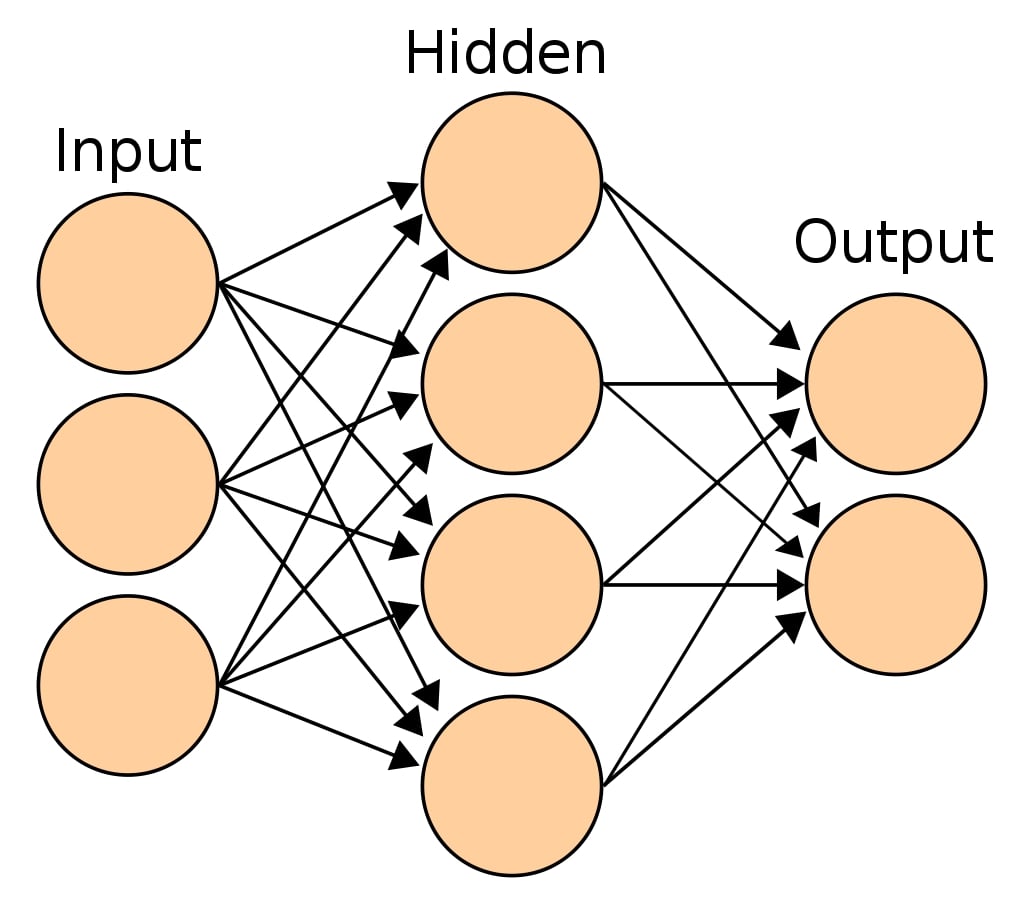
The most common type of neural network referred to as Multi-Layer Perceptron (MLP) is a function that maps input to output. MLP has a single input layer and a single output layer. In between, there can be one or more hidden layers. The input layer has the same set of neurons as that of features. Hidden layers can have more than one neuron as well. Each neuron is a linear function to which activation function is applied to solve complex problems. The output from each layer is given as input to all neurons of the next layers.
Sample Multi-Layer Perceptron
sklearn provides 2 estimators for classification and regression problems respectively.
- MLPClassifier
- MLPRegressor
We'll start by importing necessary libraries for the tutorial.
import numpy as np
import pandas as pd
import matplotlib.pyplot as plt

import sklearn

import itertools
import warnings
warnings.filterwarnings('ignore')

np.set_printoptions(precision=2)
%matplotlib inline
Load Datasets
We'll be loading below mentioned two for our purpose.
- Digits Dataset: We'll be using digits dataset which has images of size
8x8for digits0-9. We'll use digits data for classification tasks below. - Boston Housing Dataset: We'll be using the Boston housing dataset which has information about various house properties like average no of rooms, per capita crime rate in town, etc. We'll be using it for regression tasks.
Sklearn provides both of this dataset as a part of the datasets module. We can load them by calling load_digits() and load_boston() methods. It returns dictionary-like object BUNCH which can be used to retrieve features and target.
from sklearn.datasets import load_digits, load_boston

digits = load_digits()
X_digits, Y_digits = digits.data, digits.target
print('Dataset Sizes : ', X_digits.shape, Y_digits.shape)
boston = load_boston()
X_boston, Y_boston = boston.data, boston.target
print('Dataset Sizes : ', X_boston.shape, Y_boston.shape)
MLPClassifier 
MLPClassifier is an estimator available as a part of the neural_network module of sklearn for performing classification tasks using a multi-layer perceptron.
Splitting Data Into Train/Test Sets
We'll split the dataset into two parts:
Training datawhich will be used for the training model.Test dataagainst which accuracy of the trained model will be checked.
train_test_split function of model_selection module of sklearn will help us split data into two sets with 80% for training and 20% for test purposes. We are also using seed(random_state=123) with train_test_split so that we always get the same split and can reproduce results in the future as well.
Please make a note that we are also using stratify parameter which will prevent unequal distribution of all classes in train and test sets.For each classes, we'll have 80% samples in train set and 20% samples in test set. This will make sure that we don't have any dominating class in either train or test set.
from sklearn.model_selection import train_test_split

X_train, X_test, Y_train, Y_test = train_test_split(X_digits, Y_digits, train_size=0.80, test_size=0.20, stratify=Y_digits, random_state=123)
print('Train/Test Sizes : ', X_train.shape, X_test.shape, Y_train.shape, Y_test.shape)
Fitting Default Model To Train Data
We'll first fit the MLPClassifier model with default parameters to our train data.
from sklearn.neural_network import MLPClassifier

mlp_classifier  = MLPClassifier(random_state=123)
mlp_classifier.fit(X_train, Y_train)
Evaluating Trained Model On Test Data.
Almost all models in Scikit-Learn API provides predict() method which can be used to predict target variable on Test Set passed to it.
Y_preds = mlp_classifier.predict(X_test)

print(Y_preds[:15])
print(Y_test[:15])

print('Test Accuracy : %.3f'%mlp_classifier.score(X_test, Y_test)) ## Score method also evaluates accuracy for classification models.
print('Training Accuracy : %.3f'%mlp_classifier.score(X_train, Y_train))
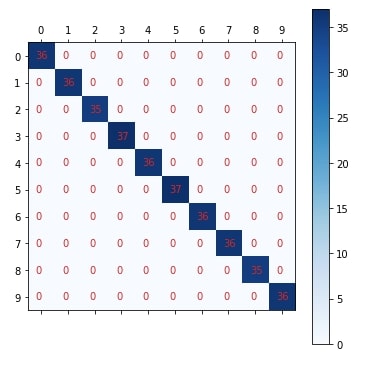
Plotting Confusion Matrix
Below we have created a method named plot_confusion_matrix() which accepts original labels of data and predicted labels by model. It then plots a confusion matrix using matplotlib. We'll be reusing the same method for plotting the confusion matrix.
from sklearn.metrics import confusion_matrix

def plot_confusion_matrix(Y_test, Y_preds):
    conf_mat = confusion_matrix(Y_test, Y_preds)
    #print(conf_mat)
    fig = plt.figure(figsize=(6,6))
    plt.matshow(conf_mat, cmap=plt.cm.Blues, fignum=1)
    plt.yticks(range(10), range(10))
    plt.xticks(range(10), range(10))
    plt.colorbar();
    for i in range(10):
        for j in range(10):
            plt.text(i-0.2,j+0.1, str(conf_mat[j, i]), color='tab:red')
plot_confusion_matrix(Y_test, mlp_classifier.predict(X_test))

Important Attributes of MLPClassifier
Below is a list of important attributes available with an MLPClassifier which can provide meaningful insights once the model is trained.
loss_- It returns loss after the training process has completed.coefs_- It returns an array of lengthn_layers-1where each element represents weights associated with layer i.intercepts_- It returns an array of lengthn_layers-1where each element represents intercept associated with layer i's perceptrons.n_iter_- The number of iterations for which estimator ran.out_activation_- It returns name of output layer activation function.
print("Loss : ", mlp_classifier.loss_)
print("Number of Coefs : ", len(mlp_classifier.coefs_))

[weights.shape for weights in mlp_classifier.coefs_]
print("Number of Intercepts : ", len(mlp_classifier.intercepts_))

[intercept.shape for intercept in mlp_classifier.intercepts_]
print("Number of Iterations for Which Estimator Ran : ", mlp_classifier.n_iter_)
print("Name of Output Layer Activation Function : ", mlp_classifier.out_activation_)
Finetuning Model By Doing Grid Search On Various Hyperparameters.
Below is a list of common hyperparameters that needs tuning for getting the best fit for our data. We'll try various hyperparameters settings to various splits of train/test data to find out best fit which will have almost the same accuracy for both train & test dataset or have quite less difference between accuracy.
- hidden_layer_sizes - It accepts tuple of integer specifying sizes of hidden layers in multi layer perceptrons. According to size of tuple, that many perceptrons will be created per hidden layer.
default=(100,) - activation - It specifies activation function for hidden layers. It accepts one of below strings as input.
default=relu'identity'- No Activation.f(x) = x'logistic'- Logistic Sigmoid Function.f(x) = 1 / (1 + exp(-x))'tanh'- Hyperbolic tangent function.f(x) = tanh(x)'relu'- Rectified Linear Unit function.f(x) = max(0, x)
- solver - It accepts one of below strings specifying which optimization solver to use for updating weights of neural network hidden layer perceptrons.
default='adam''lbfgs''sgd''adam'
- learning_rate_init - It specifies initial learning rate to be used. Based on value of this parameter weights of perceptrons are updated.
default=0.001 - learning_rate - It specifies learning rate schedule to be used for training. It accepts one of below strings as value and only applicable when
solver='sgd'.'constant'- Keeps learning rate constant through a learning process which was set inlearning_rate_init.'invscaling'- It gradually decreases learning rate.effective_learning_rate = learning_rate_init / pow(t, power_t)'adaptive'- It keeps learning rate constant as long as loss is decreasing or score is improving. If consecutive epochs fails in decreasing loss according totolparameter andearly_stoppingis on, then it divides current learning rate by5.
- batch_size - It accepts integer value specifying size of batch to use for dataset.
default='auto'. The defaultautobatch size will set batch size tomin(200, n_samples). - tol - It accepts float values specifying threshold for optimization. When training loss or score is not improved by at least
tolforn_iter_no_changeiterations, then optimization ends iflearning_rateisconstantelse it decreases learning rate iflearning_rateisadaptive.default=0.0001 - alpha - It specifies L2 penalty coefficient to be applied to perceptrons.
default=0.0001 - momentum - It specifies momentum to be used for gradient descent and accepts float value between
0-1. It's applicable when solver issgd. - early_stopping - It accepts boolean value specifying whether to stop training if training score/loss is not improving.
default=False - validation_fraction - It accepts float value between
0-1specifying amount of training data to keep aside ifearly_stoppingis set.default=0.1
GridSearchCV
It's a wrapper class provided by sklearn which loops through all parameters provided as params_grid parameter with a number of cross-validation folds provided as cv parameter, evaluates model performance on all combinations and stores all results in cv_results_ attribute. It also stores model which performs best in all cross-validation folds in best_estimator_ attribute and best score in best_score_ attribute.
n_jobs parameter is provided by many estimators. It accepts number of cores to use for parallelization. If value of -1 is given then it uses all cores. It uses joblib parallel processing library for running things in parallel in background.
We'll below try various values for the above-mentioned hyperparameters to find the best estimator for our dataset by splitting data into 5-fold cross-validation.
%%time

from sklearn.model_selection import GridSearchCV

params = {'activation': ['relu', 'tanh', 'logistic', 'identity'],
          'hidden_layer_sizes': [(100,), (50,100,), (50,75,100,)],
          'solver': ['adam', 'sgd', 'lbfgs'],
          'learning_rate' : ['constant', 'adaptive', 'invscaling']
         }

mlp_classif_grid = GridSearchCV(MLPClassifier(random_state=123), param_grid=params, n_jobs=-1, cv=5, verbose=5)
mlp_classif_grid.fit(X_train,Y_train)

print('Train Accuracy : %.3f'%mlp_classif_grid.best_estimator_.score(X_train, Y_train))
print('Test Accuracy : %.3f'%mlp_classif_grid.best_estimator_.score(X_test, Y_test))
print('Best Accuracy Through Grid Search : %.3f'%mlp_classif_grid.best_score_)
print('Best Parameters : ',mlp_classif_grid.best_params_)
Plotting Confusion Matrix
plot_confusion_matrix(Y_test, mlp_classif_grid.best_estimator_.predict(X_test))
MLPRegressor 
MLPRegressor is an estimator available as a part of the neural_network module of sklearn for performing regression tasks using a multi-layer perceptron.
Splitting Data Into Train/Test Sets
We'll split the dataset into two parts:
Train data(80%)which will be used for the training model.Test data(20%)against which accuracy of the trained model will be checked.
X_train, X_test, Y_train, Y_test = train_test_split(X_boston, Y_boston, train_size=0.80, test_size=0.20, random_state=123)
print('Train/Test Sizes : ', X_train.shape, X_test.shape, Y_train.shape, Y_test.shape)
from sklearn.neural_network import MLPRegressor

mlp_regressor  = MLPRegressor(random_state=123)
mlp_regressor.fit(X_train, Y_train)
Y_preds = mlp_regressor.predict(X_test)

print(Y_preds[:10])
print(Y_test[:10])

print('Test R^2 Score : %.3f'%mlp_regressor.score(X_test, Y_test)) ## Score method also evaluates accuracy for classification models.
print('Training R^2 Score : %.3f'%mlp_regressor.score(X_train, Y_train))
Important Attributes of MLPRegressor
MLPRegressor has all attributes the same as that of MLPClassifier.
print("Loss : ", mlp_regressor.loss_)
print("Number of Coefs : ", len(mlp_regressor.coefs_))

[weights.shape for weights in mlp_regressor.coefs_]
print("Number of Intercepts : ", len(mlp_regressor.intercepts_))

[intercept.shape for intercept in mlp_regressor.intercepts_]
print("Number of Iterations for Which Estimator Ran : ", mlp_regressor.n_iter_)
print("Name of Output Layer Activation Function : ", mlp_regressor.out_activation_)
Finetuning Model By Doing Grid Search On Various Hyperparameters.
MLPRegressor has almost the same parameters as that of MLPClassifier.
We'll below try various values for the above-mentioned hyperparameters to find the best estimator for our dataset by splitting data into 5-fold cross-validation.
%%time

params = {'activation': ['relu', 'tanh', 'logistic', 'identity'],
          'hidden_layer_sizes': list(itertools.permutations([50,100,150],2)) + list(itertools.permutations([50,100,150],3)) + [50,100,150],
          'solver': ['adam', 'lbfgs'],
          'learning_rate' : ['constant', 'adaptive', 'invscaling']
         }

mlp_regressor_grid = GridSearchCV(MLPRegressor(random_state=123), param_grid=params, n_jobs=-1, cv=5, verbose=5)
mlp_regressor_grid.fit(X_train,Y_train)

print('Train R^2 Score : %.3f'%mlp_regressor_grid.best_estimator_.score(X_train, Y_train))
print('Test R^2 Score : %.3f'%mlp_regressor_grid.best_estimator_.score(X_test, Y_test))
print('Best R^2 Score Through Grid Search : %.3f'%mlp_regressor_grid.best_score_)
print('Best Parameters : ',mlp_regressor_grid.best_params_)
Please make a note during the above experiment, we have not used sgd as the value of the solver parameter because it was exploding and pushing gradients out of limit for floating-point and failure.
This ends our small tutorial explaining neural network estimators available as a part of the sklearn. Please feel free to let us know your views in the comments section.
References 
 Sunny Solanki
Sunny Solanki
Intro: Software Developer | Youtuber | Bonsai Enthusiast
About: Sunny Solanki holds a bachelor's degree in Information Technology (2006-2010) from L.D. College of Engineering. Post completion of his graduation, he has 8.5+ years of experience (2011-2019) in the IT Industry (TCS). His IT experience involves working on Python & Java Projects with US/Canada banking clients. Since 2020, he’s primarily concentrating on growing CoderzColumn.
His main areas of interest are AI, Machine Learning, Data Visualization, and Concurrent Programming. He has good hands-on with Python and its ecosystem libraries.
Apart from his tech life, he prefers reading biographies and autobiographies. And yes, he spends his leisure time taking care of his plants and a few pre-Bonsai trees.
Contact: sunny.2309@yahoo.in


![YouTube Subscribe]() Comfortable Learning through Video Tutorials?
Comfortable Learning through Video Tutorials?
If you are more comfortable learning through video tutorials then we would recommend that you subscribe to our YouTube channel.
![Need Help]() Stuck Somewhere? Need Help with Coding? Have Doubts About the Topic/Code?
Stuck Somewhere? Need Help with Coding? Have Doubts About the Topic/Code?
 Stuck Somewhere? Need Help with Coding? Have Doubts About the Topic/Code?
When going through coding examples, it's quite common to have doubts and errors.
If you have doubts about some code examples or are stuck somewhere when trying our code, send us an email at coderzcolumn07@gmail.com. We'll help you or point you in the direction where you can find a solution to your problem.
You can even send us a mail if you are trying something new and need guidance regarding coding. We'll try to respond as soon as possible.
![Share Views]() Want to Share Your Views? Have Any Suggestions?
Want to Share Your Views? Have Any Suggestions?
 Want to Share Your Views? Have Any Suggestions?
If you want to
- provide some suggestions on topic
- share your views
- include some details in tutorial
- suggest some new topics on which we should create tutorials/blogs
 sklearn, neural-network