Scikit-Learn - Non-Linear Dimensionality Reduction: Manifold Learning¶

Table of Contents¶

• Introduction
• Isometric Mapping (Isomap)
• t-distributed Stochastic Neighbor Embedding (t-SNE)
• Spectral Embedding
• LocallyLinearEmbedding (LLE)
• Modified LLE
• Hessian LLE
• Local Tangent Space Alignment (LTSA)
• Multi-Dimensional Scaling (MDS)
• Testing Performance Of Various Dimensionality Reduction Algorithms
• References

Introduction ¶

Many real-life datasets contain non-linear features that PCA generally fails to properly detect. To solve this problem new class of algorithms called manifold learning were introduced which solves this problem of detecting non-linear features. As a part of this tutorial, we'll be introducing various manifold learning algorithms available through scikit-learn.

Below are list of manifold learning algorithms available through scikit-learn:

• Isometric Mapping (Isomap)
• t-distributed Stochastic Neighbor Embedding (t-SNE )
• Spectral Embedding
• LocallyLinearEmbedding (LLE)
• Modified LLE
• Hessian LLE
• Local Tangent Space Alignment (LTSA)
• Multi-Dimensional Scaling (MDS)

We'll be introducing the usage of each algorithm along with their important parameters, attributes, and methods available in sklearn estimators.

We'll start by importing all the necessary libraries.

Load Datasets¶

We'll start by making a s-curve dataset using the datasets module provided by scikit-learn. S-curve creates dataset in a way that 2-dimensional data is hidden into 3-dimension.

The second dataset that we'll be using is digits dataset which has images of size 8x8 for digits 0-5. We'll use digits data for classification tasks below.

Sklearn provides this dataset as a part of the datasets module. We can load it by calling load_digits() method. It returns dictionary-like object BUNCH which can be used to retrieve features and target.

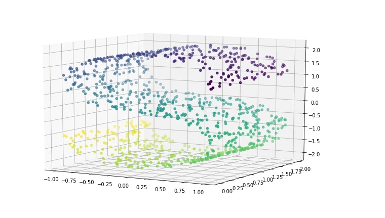
Visualizing S-Curve Dataset¶

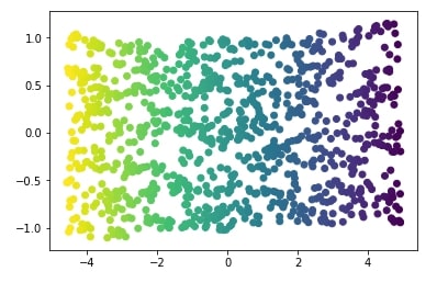
PCA Transformation Applied to S-Curve Data¶

Above s-curve hides 2-dimensional data in a 3-dimension in such a way that PCA fails to identify the structure. Below visualization of s-curve shows that PCA fails to capture information in data.

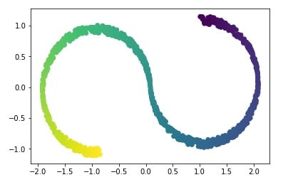
We'll try below non-linear dimensionality reduction technique called Isomap which successfully captures information in data.

Isometric Mapping (Isomap) ¶

It can be thought of as an extension of Multi-Dimensional Scaling(MDS) or Kernel PCA. It tries to find lower dimensional embedding of the original dataset while maintaining geodesic distances between all points in the original dataset. Isomap tries to get lower dimension representation of data where points maintain geodesic distance) between them like original representation. Scikit-learn provides an implementation of Isomap as a part of the manifold module.

Below is a list of important parameters of Isomap which can be tweaked to further improve performance:

• n_neighbors - It accepts integer specifying number of neighbors to consider for each point. default=5
• n_components -It accepts integer value specifying number of features transformed dataset will have.default=2
• eigen_solver -It accepts one of the below string specifying solver to use for transformation.
  • auto - Default.
  • arpack
  • dense
• path_method - It accepts one of the below string specifying method to use to find shortest path.
  • auto - Default.
  • FW - Floyd-Warshall algorithm
  • D - Dijkstra's Algorithm
• neighbors_algorithm - It accepts one of the below string specifying the algorithm to use for the nearest neighbor’s search.
  • auto - Default
  • kd_tree
  • ball_tree
  • brute
• metric - It accepts string or callable specifying metric to use when calculating distance between points. The default value is minkowski.

We'll apply Isomap to S-Curve dataset and visualize the results below.

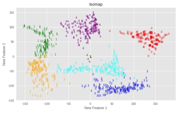
Apply Isomap to DIGITS Dataset¶

Let’s apply various manifold learning techniques to digits dataset we loaded earlier and visualize results.

Initialize Model and Transform Data¶

Plotting Transformed Dataset¶

Important Attributes of Isomap¶

Below are list of important attributes of trained Isomap instance which can provide meaningful insights:

• embedding_ - It returns embedding vector obtained through training.
• kernel_pca_ - It returns KernelPCA object used for generating embedding.
• nbrs_ - It returns nearest neighbor instance.
• dist_matrix_ - It returns geodesic distance matrix for train data.

Transform DIGITS Dataset to 3-Components Dataset using Isomap¶

t-distributed Stochastic Neighbor Embedding (t-SNE) ¶

t-SNE transforms linking between point which is represented by Gaussian joint probabilities to student's t-distributions in embedded space. It's best suited to handle data with more than one fold whereas algorithms like Isomap, LLE, etc are best suited for single fold data. t-SNE tries to group samples based on their local structure. Scikit-learn provides the TSNE estimator as a part of the manifold module to use this algorithm in practice.

Below is a list of important parameters of TSNE which can be tweaked to improve performance of the default model:

• n_components -It accepts integer value specifying number of features transformed dataset will have.default=2
• perplexity - It accepts float specifying a number of nearest neighbors used on other manifold learning algorithms. It's advised to use a value between 5-50. default=30
• early_exaggeration - It accepts float value specifying how far clusters are in embedded space.default=12
• learning_rate - It accepts float specifying learning rate of t-SNE. It's advisable to use values between 10-1000. default=200
• metric - It accepts a string or callable specifying metric to use to measure the distance between data points. default=euclidean.

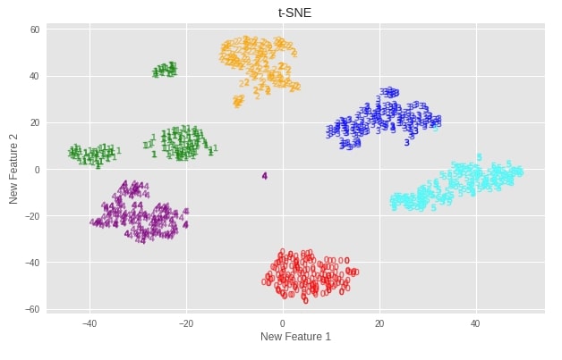
Apply t-SNE to DIGITS Dataset¶

Initialize Model and Transform Data¶

Plotting Transformed Dataset¶

Important Attributes of t-SNE¶

Below is a list of important attributes of trained t-SNE instance which can provide meaningful insights:

• embedding_ - It returns embedding vector obtained through training.
• kl_divergence_ - It returns Kullback-Leibler divergence after optimization.

Transform DIGITS Dataset to 3-Components Dataset using t-SNE¶

Spectral Embedding ¶

Spectral embedding finds a low dimensional representation of data using spectral decomposition of graph Laplacian. Scikit-Learn provides SpectralEmbedding implementation as a part of the manifold module.

Below is a list of important parameters of TSNE which can be tweaked to improve performance of the default model:

• n_components -It accepts integer value specifying number of features transformed dataset will have.default=2
• affinity - It accepts a string or callable specifying how to calculate the affinity matrix of data. The affinity matrix has a size of (n_samples x n_samples). Below is a list of possible values for it.
  • nearest_neighbors - Default.
  • rbf
  • precomputed
  • precomputed_nearest_neighbors
• gamma - It accepts float value specifying gamma parameter to use when affinity is set to rbf.
• n_neighbors -It accepts integer value specifying number of neighbors to use when affinity is set to nearest_neighbors.

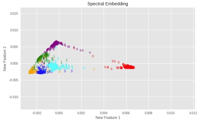
Apply Spectral Embedding to DIGITS Dataset¶

Initialize Model and Transform Data¶

Plotting Transformed Dataset¶

Important Attributes of Spectral Embedding¶

Below is a list of important attributes of trained Spectral Embedding instance which can provide meaningful insights:

• embedding_ - It returns embedding vector obtained through training.
• affinity_matrix_ - It returns affinity matrix calculated.

Transform DIGITS Dataset to 3-Components Dataset using Spectral Embedding¶

LocallyLinearEmbedding (LLE) ¶

LLE tries to find the lower-dimensional projection of data while maintaining distances within local neighborhood points. It can be viewed as applying a series of local PCAs that are then compared globally to find the most suited non-linear embedding. As an algorithm based on neighborhood points, we need to provide a number of neighbors to consider for it as input parameter (n_neighbors). Scikit-learn provides an estimator named LocallyLinearEmbedding as a part of the manifold module for performing Locally Linear Embedding on data.

Below is a list of important parameters of LocallyLinearEmbedding which can be tweaked to further improve performance:

• n_neighbors - It accepts integer specifying number of neighbors to consider for each point. default=5
• n_components -It accepts integer value specifying number of features transformed dataset will have.default=2
• eigen_solver -It accepts one of the below string specifying solver to use for transformation.
  • auto - Default.
  • arpack
  • dense
• method - This parameter accepts string value specifying different variants of LLE. Below are list of possible values.
  • standard - Default.
  • hessian
  • modified
  • ltsa
• neighbors_algorithm - It accepts one of the below string specifying algorithm to use for nearest neighbors search.
  • auto - Default
  • kd_tree
  • ball_tree
  • brute

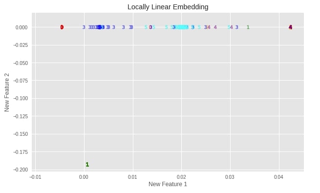
Apply LLE to DIGITS Dataset¶

Initialize Model and Transform Data¶

Plotting Transformed Dataset¶

Important Attributes of LLE¶

Below is a list of important attributes of trained LLE instance which can provide meaningful insights:

• embedding_ - It returns embedding vector obtained through training.
• reconstruction_error_ - It returns float value specifying reconstruction error associated with embedding.
• nbrs_ - It returns nearest neighbor instance.

Transform DIGITS Dataset to 3-Components Dataset using LLE¶

Modified LLE ¶

LLE suffers from a regularization problem when a number of neighbors are greater than a number of input dimensions. To solve this problem and apply regularization sklearn provides a modified version of LLE as well. The developer needs to supply the method as "modified" to use this version of LLE when calling LocallyLinearEmbedding estimator of the manifold module.

It required a number of neighbors greater than a number of features.

The parameters of Modified LLE are the same as Standard LLE due to the usage of the same estimator from sklearn.

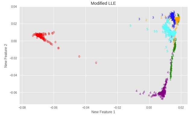
Apply Modified LLE to DIGITS Dataset¶

Initialize Model and Transform Data¶

Plotting Transformed Dataset¶

Important Attributes of Modified LLE¶

Modified LLE has the same attributes as standard LLE.

Transform DIGITS Dataset to 3-Components Dataset using Modified LLE¶

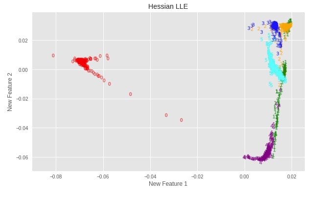
Hessian LLE ¶

Hessian is another method available with LLE to solve the regularization problem. sklearn provides this variant by setting the method parameter as "hessian" in LocallyLinearEmbedding constructor.

It requires that (number of neighbors) > (number of features) * (number of features + 3) / 2

The parameters of Hessian LLE are the same as Standard LLE due to usage of the same estimator from sklearn.

Apply Hessian LLE to DIGITS Dataset¶

Initialize Model and Transform Data¶

Plotting Transformed Dataset¶

Important Attributes of Hessian LLE¶

Hessian LLE has the same attributes as standard LLE.

Transform DIGITS Dataset to 3-Components Dataset using Hessian LLE¶

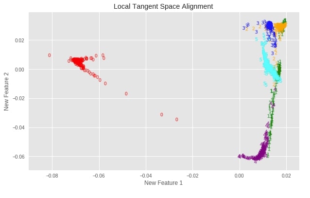
Local Tangent Space Alignment (LTSA) ¶

LTSA is not variant of LLE but it is the same algorithmically to LLE. Unlike LLE, LTSA tries to maintain local geometry at each neighborhood via its tangent space and then optimizes to align these tangent spaces to generate embeddings for data. Scikit-learn provides this variant by setting the method parameter as "ltsa" in LocallyLinearEmbedding constructor.

The parameters of LTSA are the same as Standard LLE due to usage of the same estimator from sklearn.

Apply LTSA to DIGITS Dataset¶

Initialize Model and Transform Data¶

Plotting Transformed Dataset¶

Important Attributes of LTSA¶

LTSA has the same attributes as standard LLE.

Transform DIGITS Dataset to 3-Components Dataset using LTSA¶

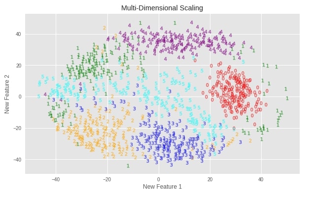
Multi-Dimensional Scaling (MDS) ¶

Multi-Dimensional Scaling an algorithm used for analyzing similarity or dissimilarity in data. It tries to decide similarity or dissimilarity based on distances between data points in geometric spaces. It tries to find a low dimensional representation of data that maintains the same distance between data points in original high dimensional data. Scikit-learn provides an implementation of MDS as a part of manifold module.

Below is a list of important parameters of MDS which can be tweaked to further improve performance:

• n_components -It accepts integer value specifying number of features transformed dataset will have.default=2
• metric - It accepts boolean value specifying to perform metric MDS if set to True else use nonmetric MDS.
• dissimilarity - It accepts string value specifying dissimilarity measure.
  • euclidean - Default.
  • precomputed
• eps - It accepts float value specifying relative tolerance with respect to stress.default=0.001

Apply MDS to DIGITS Dataset¶

Initialize Model and Transform Data¶

Plotting Transformed Dataset¶

Important Attributes of MDS¶

Below is a list of important attributes of trained MDS instance which can provide meaningful insights:

• embedding_ - It returns embedding vector obtained through training.
• stress_ - It returns the sum of squared distance for disparities and distances for all constrained points.

Transform DIGITS Dataset to 3-Components Dataset using MDS¶

Testing Performance Of Various Dimensionality Reduction Algorithms ¶

Below we have designed a method named test_model which takes as input classifier, data, and labels as input. It then divides data into train/test sets, train a classifier on train data, and evaluate it on both train & test data. It prints the accuracy of the classifier on both train and test data.

The second method that we have declared tries classifier passed to it on all 2-component and 3-component transformation of the original digits dataset. It prints the classifier's accuracy on all transformed datasets to check which one performs well like original and succeeded in keeping as much information from original high-dimensional data. It also tries classifiers on original data.

We are calling compare_accuracy_of_various_techniques() method with 2 different classifiers:

• LogisticRegression
• KNeighborsClassifier

This ends our small tutorial explaining various estimators available for performing unsupervised manifold learning dimensionality reduction with sklearn. Please feel free to let us know your views in the comments section.

References ¶

• Scikit-Learn - Linear Dimensionality Reduction : PCA
• Scikit-Learn Docs - Manifold Learning