Scikit-Learn - Linear Dimensionality Reduction: Principal Component Analysis
Table of Contents
- Introduction
- Principal Component Analysis (PCA)
- Comparing Performance of Datasets With PCA Applied
- References
Introduction 
The type of Unsupervised learning which is quite interesting is dimensionality reduction. It results in the reduction of dimensions of data hence in effect reduces data size as well.
There are major 2 types of dimensionality reduction techniques.
- Linear Projection of Data (Principal Component Analysis, Independent Component Analysis, Linear Discriminant Analysis, etc. )
- Non-Linear Projection of Data (Manifold Learning - Isomap, TSNE, SpectralEmbedding, MDS, LocallyLinearEmbedding)
We'll be discussing Linear Dimensionality Reduction in this tutorial (PCA) and algorithms available for it in scikit-learn. We'll not go much into theoretical depth of concept but will try to explain the usage of algorithms available in scikit-learn about it.
We'll start by importing related libraries.
import numpy as np
import pandas as pd
import matplotlib.pyplot as plt
from mpl_toolkits.mplot3d import Axes3D

import sklearn

import sys
import warnings

warnings.filterwarnings('ignore')

print("Python Version : ",sys.version)
print("Scikit-Learn Version : ",sklearn.__version__)

%matplotlib inline
Principal Component Analysis (PCA) 
PCA is a linear projection of data into new feature space different from the original one. In PCA, We find new features for representing data which linear combinations of old data but less in terms of dimensions. One can also say that we rotate data into a new feature space with fewer dimensions.
The main concept behind PCA is to reduce the dimensions of data while capturing most of the information of data. PCA finds these features by looking at the direction of maximum variance and keeping only features which present maximum variance in data. It results in finding a dataset which is low in size but still possess the same information as that of the original dataset.
It helps in the reduction of computation time for ML algorithms, reduction of storage memory, and also helps to fight "Curse of Dimensionality".
Load IRIS Dataset 
Below we are loading the IRIS dataset which comes as default with the sklearn package. It returns Bunch object which is almost the same as the dictionary. We'll also print details about the dataset.
from sklearn import datasets

iris = datasets.load_iris()

print('Dataset features names : '+str(iris.feature_names))
print('Dataset features size : '+str(iris.data.shape))
print('Dataset target names : '+str(iris.target_names))
print('Dataset target names : '+str(iris.target.shape))

X_iris, Y_iris = iris.data, iris.target
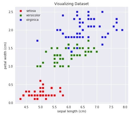
Visualizing Data 
Below we are visualizing our data by using a scatter plot which shows the relationship between two attributes of data (sepal length - X-axis vs petal width- Y-axis). One can also try different combinations of attributes of data to see how they are related. We also have color-encoded classes.
with plt.style.context(('ggplot','seaborn')):
    plt.figure(figsize=(15,6))
    plt.subplot(121)
    for i,c in [(0,'red'),(1,'green'),(2,'blue')]:
        plt.scatter(iris.data[iris.target==i,0],iris.data[iris.target==i,3], c=c, s=40, marker='s', label=iris.target_names[i])
    plt.xlabel(iris.feature_names[0])
    plt.ylabel(iris.feature_names[3])
    plt.legend(loc='best')
    plt.title('Visualizing Dataset')
Initializing PCA & Fitting To Data 
Below we'll initialize 2 different versions of PCA (One with 2 components and another with 3 components). We'll then fit data to both of these models. Here n_components parameter refers to a number of features we want into a transformed dataset.
from sklearn import decomposition

pca2 = decomposition.PCA(n_components=2)
pca3 = decomposition.PCA(n_components=3)
pca2.fit(X_iris), pca3.fit(X_iris)
Transforming Data To New Dimensions 
Once a model has been fit to data, it can then be used to transform the dataset into a new dimensional space defined as a number of components when initializing the model. We'll create 2 transformed datasets(one with 2 features and one with 3 features) from the original IRIS dataset.
X_iris_pca2 = pca2.transform(X_iris)
X_iris_pca3 = pca3.transform(X_iris)

print('New Dataset size after transformations : ', X_iris_pca2.shape, X_iris_pca3.shape)
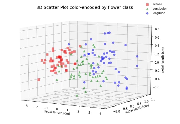
Plotting Transformed Datasets 
We'll try to visualize both transformed datasets using scatter charts and color-encode them using flower class. It'll help us understand whether the transformed dataset also has the same spread of data as that of the original.
fig = plt.figure(1, figsize=(8, 6))

colors = ['red','green','blue']
markers = ['s','^','o']

with plt.style.context(('seaborn','ggplot')):
    for iris_class in range(3):
        plt.scatter(X_iris_pca2[Y_iris==iris_class,0],X_iris_pca2[Y_iris==iris_class,1],\
                   c=colors[iris_class], label=iris.target_names[iris_class], marker=markers[iris_class], s=50, alpha=0.5)
    plt.legend(loc="best")
    plt.title('Scatter Plot of Feature-1 vs Feauter-2 color-encoded by flower class')
    plt.xlabel("New Feature 1")
    plt.ylabel("New Feature 2")

fig = plt.figure(1, figsize=(8, 6))
ax = Axes3D(fig)

colors = ['red','green','blue']
markers = ['s','^','o']

with plt.style.context(('seaborn','ggplot')):
    for iris_class in range(3):
        ax.scatter3D(X_iris_pca3[Y_iris==iris_class,0],X_iris_pca3[Y_iris==iris_class,1],X_iris_pca3[Y_iris==iris_class,2], \
                   c=colors[iris_class], label=iris.target_names[iris_class], marker=markers[iris_class], s=50, alpha=0.5)
    ax.legend(loc="best")
    ax.set_title('3D Scatter Plot color-encoded by flower class')
    ax.set_xlabel(iris.feature_names[0])
    ax.set_ylabel(iris.feature_names[1])
    ax.set_zlabel(iris.feature_names[2])
    ax.view_init(10, -60);
Important Attributes of PCA 
components_It represents the direction of maximum variance in data.explained_variance_The amount of variance explained by each component.explained_variance_ratio_The percentage of variance explained by each component.singular_values_It represents singular values for each components.noise_variance_It represents estimated noise covariance.
print("PCA(2-Components) components : ", pca2.components_)
print("PCA(3-Components) components: ", pca3.components_)
print("PCA(2-components) explained variance:",pca2.explained_variance_)
print("PCA(3-components) explained variance:",pca3.explained_variance_)
print("PCA(2-components) explained variance ratio:",pca2.explained_variance_ratio_)
print("PCA(3-components) explained variance ratio:",pca3.explained_variance_ratio_)
print("PCA(2-components) singular values :",pca2.singular_values_)
print("PCA(3-components) singular values :",pca3.singular_values_)
print("PCA(2-components) noise variance :",pca2.noise_variance_)
print("PCA(3-components) noise variance :",pca3.noise_variance_)
Load DIGITS Dataset 
We'll try PCA on digits datasets as well which is available in the scikit-learn library. We'll be loading only 6 classes instead of loading all 10-classes of digits as it'll help us clearly see classes in plotted data. Below we are loading digits dataset which is readily available in sklearn.
digits = datasets.load_digits(n_class=6)

X_digits, Y_digits  = digits.data, digits. target
print('Dataset Size : ', X_digits.shape, Y_digits.shape)
Please make a note that the digits dataset has 64 features as each image is of size 8x8 pixels.
Transforming Data To New Dimensions 
We'll be transforming digits dataset to 2-features and 3-features dataset from 64 features dataset which is quite a big reduction in the size of data. We'll also lose some important information when decreasing dataset features by such margin and will impact our classification accuracy as well in the future.
We are using the fit_transform() method available for PCA to perform both fit and transform functionalities together.
X_digits_pca2 = pca2.fit_transform(X_digits)
X_digits_pca3 = pca3.fit_transform(X_digits)

print('Transformed Data sizes : ', X_digits_pca2.shape, X_digits_pca3.shape)
Plotting Transformed DIGITS datasets 
Below we are using scatter charts to visualize 2-features and 3-features PCA transformed digits datasets. We have also color-encoded each digit to differentiate them from one another.
with plt.style.context(('seaborn','ggplot')):
    fig = plt.figure(1, figsize=(10, 5))

    colors = ['red','green','yellow','blue','purple','cyan','magenta', 'firebrick', 'lawngreen','indigo']
    for digit in range(0,6):
        plt.scatter(X_digits_pca2[Y_digits==digit,0],X_digits_pca2[Y_digits==digit,1], c = colors[digit], marker="$"+str(digit)+"$",s =50, alpha=0.5)
    plt.xlabel("New Feature 1")
    plt.ylabel("New Feature 2")
    plt.title('Scatter Plot representing various digits')
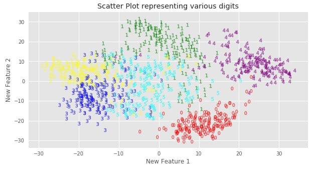
We can clearly see that classes are still separate from each other even after dimensionality reduction. It seems that PCA has tried to maintain as much information about the dataset even after doing a reduction in a number of features.
fig = plt.figure(1, figsize=(10, 8))
ax = Axes3D(fig)

colors = ['red','green','yellow','blue','purple','cyan','magenta', 'firebrick', 'lawngreen','indigo']

with plt.style.context(('seaborn','ggplot')):
    for digit in range(6):
        ax.scatter3D(X_digits_pca3[Y_digits==digit,0],X_digits_pca3[Y_digits==digit,1],X_digits_pca3[Y_digits==digit,2], \
                   c=colors[digit], marker="$"+str(digit)+"$", s=50, alpha=0.5)
    ax.view_init(10, -60)
    ax.set_title('3D Scatter Plot color-encoded by digits')
    ax.set_xlabel('Feature 1')
    ax.set_ylabel('Feature 2')
    ax.set_zlabel('Feature 3')
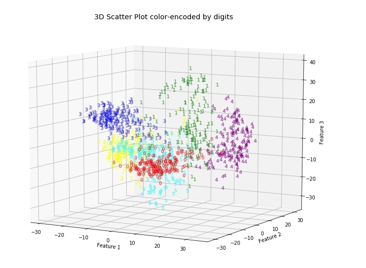
Make a note that we determined these new features without any information about labels of data, hence it's unsupervised learning. PCA gives insight into the distribution of data for different classes.
Comparing Performance of Datasets With PCA Applied 
Below we are checking the performance of LinearRegression and KNeighborsClassifier models on original IRIS and digits datasets as well as on PCA transformed datasets to see whether the decrease in dimensions has resulted in the loss of information which impacts the performance of classifier a lot.
We have created a generic method that takes as input classifier and dataset along with the target. It then splits the dataset into train/test sets, fit classifier into train data, and evaluate the test set. It also prints the model's performance on both train and test sets.
from sklearn.model_selection import train_test_split

def test_model(classifier, X, Y):
    X_train, X_test, Y_train, Y_test = train_test_split(X, Y, train_size=0.80, test_size=0.20, stratify=Y, random_state=123)
    print("Dataset Size : ",sys.getsizeof(X),"bytes, Shape : ", X_train.shape, X_test.shape, Y_train.shape, Y_test.shape)
    classifier.fit(X_train, Y_train)
    print('Train Accuracy : %.2f, Test Accuracy : %.2f'%(classifier.score(X_train, Y_train), classifier.score(X_test, Y_test)))


def compare_accuracy_of_various_techniques(classifier):
    print("Iris dataset performance without PCA :")
    test_model(classifier, X_iris, Y_iris)
    print("\nIris dataset performance with PCA(2 components) :")
    test_model(classifier, X_iris_pca2, Y_iris)
    print("\nIris dataset performance with PCA(3 components) :")
    test_model(classifier, X_iris_pca3, Y_iris)
    print("\nDigits dataset performance without PCA :")
    test_model(classifier, X_digits, Y_digits)
    print("\nDigits dataset performance with PCA(2 components) :")
    test_model(classifier, X_digits_pca2, Y_digits)
    print("\nDigits dataset performance with PCA(3 components) :")
    test_model(classifier, X_digits_pca3, Y_digits)
from sklearn.linear_model import LogisticRegression

classifier = LogisticRegression(solver='newton-cg',multi_class='auto')
compare_accuracy_of_various_techniques(classifier)
from sklearn.neighbors import KNeighborsClassifier

classifier = KNeighborsClassifier()
compare_accuracy_of_various_techniques(classifier)
We can notice from the above analysis that the accuracy of the DIGITS dataset is impacted quite more compared to that of the IRIS dataset after performing dimensionality reduction using PCA. We had reduced the size of DIGITS by quite a margin which has resulted in a loss of information. One can decide how many components to use as a parameter of PCA by checking model accuracy on a various number of features.
We can also use PCA Component Explained Variance Chart to decide how many features we can let go which will not result in information getting lost. The PCA components explained variance chart let us know how much of the original data variance is contained within first n_components.
This ends our small tutorial introducing the usage of PCA using scikit-learn. Please feel free to let us know your views in the comments section.
References 
 Sunny Solanki
Sunny Solanki
Intro: Software Developer | Youtuber | Bonsai Enthusiast
About: Sunny Solanki holds a bachelor's degree in Information Technology (2006-2010) from L.D. College of Engineering. Post completion of his graduation, he has 8.5+ years of experience (2011-2019) in the IT Industry (TCS). His IT experience involves working on Python & Java Projects with US/Canada banking clients. Since 2020, he’s primarily concentrating on growing CoderzColumn.
His main areas of interest are AI, Machine Learning, Data Visualization, and Concurrent Programming. He has good hands-on with Python and its ecosystem libraries.
Apart from his tech life, he prefers reading biographies and autobiographies. And yes, he spends his leisure time taking care of his plants and a few pre-Bonsai trees.
Contact: sunny.2309@yahoo.in


![YouTube Subscribe]() Comfortable Learning through Video Tutorials?
Comfortable Learning through Video Tutorials?
If you are more comfortable learning through video tutorials then we would recommend that you subscribe to our YouTube channel.
![Need Help]() Stuck Somewhere? Need Help with Coding? Have Doubts About the Topic/Code?
Stuck Somewhere? Need Help with Coding? Have Doubts About the Topic/Code?
 Stuck Somewhere? Need Help with Coding? Have Doubts About the Topic/Code?
When going through coding examples, it's quite common to have doubts and errors.
If you have doubts about some code examples or are stuck somewhere when trying our code, send us an email at coderzcolumn07@gmail.com. We'll help you or point you in the direction where you can find a solution to your problem.
You can even send us a mail if you are trying something new and need guidance regarding coding. We'll try to respond as soon as possible.
![Share Views]() Want to Share Your Views? Have Any Suggestions?
Want to Share Your Views? Have Any Suggestions?
 Want to Share Your Views? Have Any Suggestions?
If you want to
- provide some suggestions on topic
- share your views
- include some details in tutorial
- suggest some new topics on which we should create tutorials/blogs
 sklearn-, linear-dimensionality-reduction-pca