Scikit-Learn - Hierarchical Clustering
Table of Contents
- Introduction
- scipy.hierarchy
- Scikit-Learn
- Create Moons Dataset (Two Interleaving Circles)
- Create Dataset Of Circles (Large Circle Containing A Smaller Circle)
- Create Isotropic Gaussian Blobs dataset
- Create Isotropic Gaussian Blobs dataset & Skew Blobs Using Transformation
- References
Introduction 
A clustering algorithm like KMeans is good for clustering tasks as it is fast and easy to implement but it has limitations that it works well if data can be grouped into globular or spherical clusters and also one needs to provide a number of clusters. As KMeans is based on distance from the cluster center to point in the cluster, it'll be able to cluster data that is organized globular/spherical shape and will fail to cluster data organized in a different manner.
We'll look at hierarchical methods in this tutorial.
Hierarchical Clustering
Hierarchical clustering is a kind of clustering that uses either top-down or bottom-up approach in creating clusters from data. It either starts with all samples in the dataset as one cluster and goes on dividing that cluster into more clusters or it starts with single samples in the dataset as clusters and then merges samples based on criteria to create clusters with more samples.
We can visualize the results of clustering as a dendrogram as hierarchical clustering progress. This helps us in deciding when we want to stop clustering further (how "deep") by setting "depth" with some threshold.
It has 2 types
- Agglomerative Clustering (bottom-up approach) - We start with single samples and clusters and keep on combining them into clusters until we are left with a single cluster.
- Divisive Clustering (top-down approach) - We start with the whole dataset as one cluster and then keep on dividing it into small clusters until each consists of a single sample.
To understand agglomerative clustering & divisive clustering, we need to understand concepts of single linkage and complete linkage. Single linkage helps in deciding the similarity between 2 clusters which can then be merged into one cluster. Complete linkage helps with divisive clustering which is based on dissimilarity measures between clusters. Divisive Clustering chooses the object with the maximum average dissimilarity and then moves all objects to this cluster that are more similar to the new cluster than to the remainder.
- Single Linkage: We take pairs of most similar samples in each cluster and merge 2 clusters that have the most similar 2 members into the new cluster.
- Complete Linkage: We take pairs of most dissimilar samples in each cluster and then merge them into 2 clusters where dissimilarity distance is least.
- Average Linkage: We take pairs of most similar samples in each cluster using average distance and merge 2 clusters which have the most similar 2 members into the new cluster.
- Ward: Minimizes the sum of squared distance between all pairs of clusters. Its concept is the same as KMeans but the approach is hierarchical.
Note that we measure similarity based on the distance which is generally euclidean distance.
We'll start by importing necessary libraries. We'll be explaining the usage of agglomerative clustering using scipy and scikit-learn both.
import numpy as np
import pandas as pd
import matplotlib.pyplot as plt

import scipy
from scipy.cluster import hierarchy

import sklearn

import sys

print("Python Version : ", sys.version)
print("Scikit-Learn Version : ", sklearn.__version__)
Load IRIS Data
We'll start by loading the famous IRIS dataset which has information about 3 different IRIS flower categories as features. It also holds information about the flower category. Scikit-Learn provides this dataset as part of its datasets module. We are taking only two features from the dataset for explanation purposes.
from sklearn import datasets

iris = datasets.load_iris()
X, Y = iris.data[:, [2,3]], iris.target

print("Dataset Features : ", iris.feature_names)
print("Dataset Target : ", iris.target_names)
print('Dataset Size : ', X.shape, Y.shape)
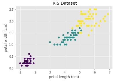
Below we are visualizing the iris dataset where the X-axis represents the 1st component (petal length) of the dataset and the Y-axis represents 2nd component (petal width). We have also color-encoded points according to flower type. We can notice that one type of flower is totally independent of the other two flowers. The flowers represented with color green and yellow overlap a bit.
with plt.style.context("ggplot"):
    plt.scatter(X[:,0], X[:, 1], c=Y)
    plt.xlabel(iris.feature_names[2])
    plt.ylabel(iris.feature_names[3])
    plt.title("IRIS Dataset")
scipy.hierarchy 
The hierarchy module of scipy provides us with linkage() method which accepts data as input and returns an array of size (n_samples-1, 4) as output which iteratively explains hierarchical creation of clusters.
The array of size (n_samples-1, 4) is explained as below with the meaning of each column of it. We'll be referring to it as an array Z of size (n_samples-1, 4).
- 0th Column - The data in this column represents cluster number at iteration
iwhich will be combined with another cluster. - 1st Column - The data in this column represents cluster number at iteration
iwhich will be combined with another cluster. - 2nd Column - The data in this column represents
distancebetween clusters specified in0thand1stcolumn. - 3rd Column - The number of original observations in this newly formed cluster.
At ith-iteration of clustering algorithm, clusters Z[i,0] and Z[i, 1] are combined to form cluster n_samples+i. A cluster with index n_samples corresponds to a cluster with the original sample.
Important Parameters of linkage()
Below is a list of other important parameters of method linkage():
- method: It accepts a string specifying linkage algorithm to use for clustering. Below is list of string arguments which it accepts.
- complete
- single
- average
- ward
- centroid
- weighted
- median
- metric: It accepts string specifying distance calculation between two points. It's set to
euclideanby default. - optimal_ordering: Its a boolean parameter which if set to True will try to minimize the distance between successive leaves.
Hierarchical Clustering - Complete Linkage 
Below we are generating cluster details for iris dataset loaded above using linkage() method of scipy.hierarchy. We have used the linkage algorithm complete for this purpose.
clusters = hierarchy.linkage(X, method="complete")

clusters[:10]
Visualizing Hierarchical Clustering as Dendrogram
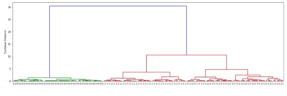
The scipy.hirearchy module provides method named dendrogram() for visualization of dendrogram created by linkage() method of clustering. It'll display overall process of how labels were combined to create clusters. Below we are visualizing dendrogram created using the complete linkage algorithm above. We need to pass it the output of the linkage() method along with original cluster labels.
def plot_dendrogram(clusters):
    plt.figure(figsize=(20,6))
    dendrogram = hierarchy.dendrogram(clusters, labels=Y, orientation="top",leaf_font_size=9, leaf_rotation=360)
    plt.ylabel('Euclidean Distance');

plot_dendrogram(clusters)
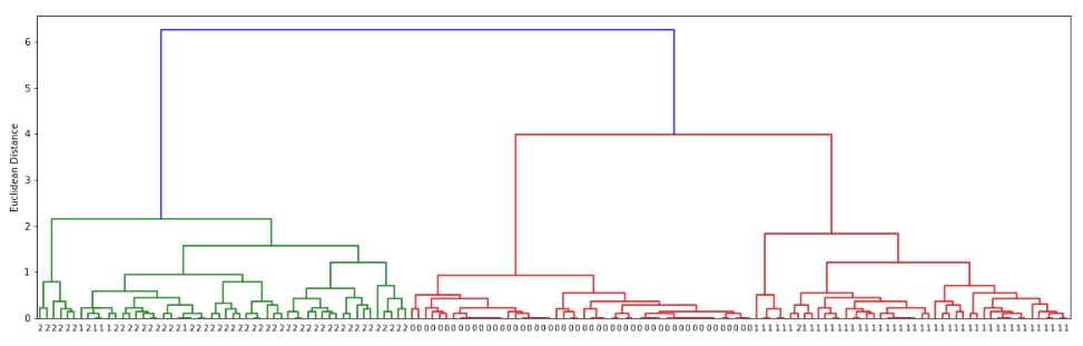
We can notice from the above visualization that the majority of labels that are from the same flower class are kept together in the same cluster. There are few errors though due to overlap in feature values as depicted in the original visualization of the dataset at the beginning.
Hierarchical Clustering - Single Linkage 
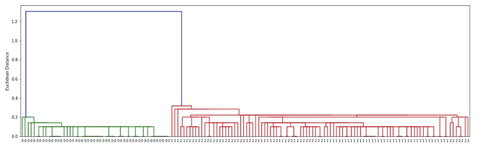
Below we are generating cluster details for iris dataset loaded above using linkage() method of scipy.hierarchy. We have used the linkage algorithm single for this purpose.
clusters = hierarchy.linkage(X, method="single")

clusters[:5]
Visualizing Hierarchical Clustering as Dendrogram
plot_dendrogram(clusters)
Hierarchical Clustering - Average Linkage 
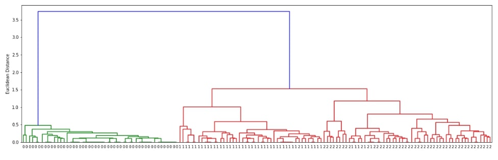
Below we are generating cluster details for iris dataset loaded above using linkage() method of scipy.hierarchy. We have used the linkage algorithm average for this purpose.
clusters = hierarchy.linkage(X, method="average")

clusters[:5]
Visualizing Hierarchical Clustering as Dendrogram
plot_dendrogram(clusters)
Hierarchical Clustering - Ward Linkage 
Below we are generating cluster details for iris dataset loaded above using linkage() method of scipy.hierarchy. We have used the linkage algorithm ward for this purpose.
clusters = hierarchy.linkage(X, method="ward")

clusters[:5]
Visualizing Hierarchical Clustering as Dendrogram
plot_dendrogram(clusters)
Scikit-Learn 
The scikit-learn also provides an algorithm for hierarchical agglomerative clustering. The AgglomerativeClustering class available as a part of the cluster module of sklearn can let us perform hierarchical clustering on data. We need to provide a number of clusters beforehand
Important Parameters of AgglomerativeClustering
Below is a list of important parameters of AgglomerativeClustering which can be tuned to improve the performance of the clustering algorithm:
- linkage - It accepts string specifying linkage algorithms to use for clustering. It has a
wardas the default value. Below is a list of values that this parameter accepts.- single
- complete
- average
- ward
- affinity - It accepts string value or function specifying metric used to calculate linkage distance between points. The default value is
euclideanfor it. Below is a list of possible values.- euclidean
- l1
- l2
- manhattan
- cosine
- precomputed
Agglomerative Clustering - Ward 
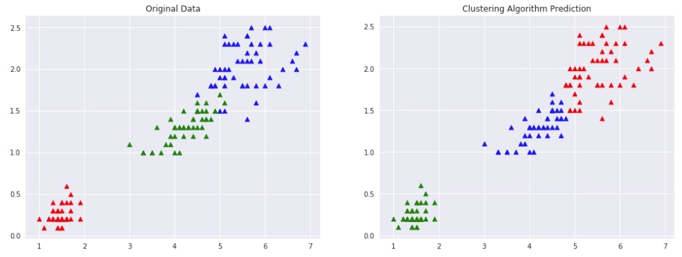
Below we are trying AgglomerativeClustering on IRIS data loaded earlier with linkage algorithm as ward. We'll fit the model on train data and predict labels using the fit_predict() method. We'll be using the default euclidean method of measuring distance between two points of data.
from sklearn.cluster import AgglomerativeClustering

clustering = AgglomerativeClustering(n_clusters=3, linkage="ward")
Y_preds = clustering.fit_predict(X)

Y_preds
Evaluating Performance Of Clustering Algorithm
We'll be using the adjusted_rand_score method for measuring the performance of the clustering algorithm by giving original labels and predicted labels as input to the method. It tries all possible pairs of clustering labels returns a value between -1.0 and 1.0. If the clustering algorithm has predicted labels randomly then it'll return value of 0.0. If the value of 1.0 is returned then it means that the algorithm predicted all labels correctly.
from sklearn.metrics import adjusted_rand_score

adjusted_rand_score(Y, Y_preds)
Visualizing Original and Predicted Labels for Comparison
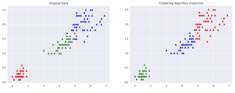
Below we have designed a method that takes as input original data, original labels, predicted labels and then plots two scatter plot comparing original data with predicted labels. This plot can help us compare the result of the clustering algorithm by comparing points to check whether they have been assigned the same cluster (flower type) as original data.
def plot_actual_prediction_iris(X, Y, Y_preds):
    with plt.style.context(("ggplot", "seaborn")):
        plt.figure(figsize=(17,6))

        plt.subplot(1,2,1)
        plt.scatter(X[Y==0,0],X[Y==0,1], c = 'red', marker="^", s=50)
        plt.scatter(X[Y==1,0],X[Y==1,1], c = 'green', marker="^", s=50)
        plt.scatter(X[Y==2,0],X[Y==2,1], c = 'blue', marker="^", s=50)
        plt.title("Original Data")

        plt.subplot(1,2,2)
        plt.scatter(X[Y_preds==0,0],X[Y_preds==0,1], c = 'red', marker="^", s=50)
        plt.scatter(X[Y_preds==1,0],X[Y_preds==1,1], c = 'green', marker="^", s=50)
        plt.scatter(X[Y_preds==2,0],X[Y_preds==2,1], c = 'blue', marker="^", s=50)

        plt.title("Clustering Algorithm Prediction");

plot_actual_prediction_iris(X, Y, Y_preds)
Agglomerative Clustering - Single Linkage 
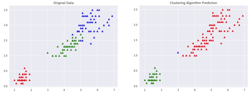
Below we are trying AgglomerativeClustering on IRIS data loaded earlier with linkage algorithm as single. We'll fit the model on train data and predict labels using the fit_predict() method. We'll be using the default euclidean method of measuring distance between two points of data.
We are then plotting data with original labels and predicted labels to compare the performance of the clustering algorithm.
clustering = AgglomerativeClustering(n_clusters=3, linkage="single")
Y_preds = clustering.fit_predict(X)

Y_preds
Evaluating Performance Of Clustering Algorithm
adjusted_rand_score(Y, Y_preds)
Visualizing Original and Predicted Labels for Comparison
plot_actual_prediction_iris(X, Y, Y_preds)
Agglomerative Clustering - Complete Linkage 
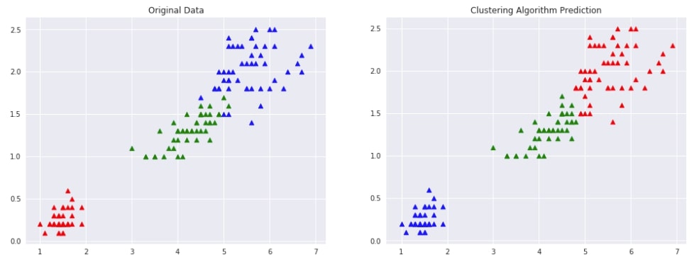
Below we are trying AgglomerativeClustering on IRIS data loaded earlier with the linkage algorithm as complete. We'll fit the model on train data and predict labels using the fit_predict() method. We'll be using the default euclidean method of measuring distance between two points of data.
We are then plotting data with original labels and predicted labels to compare the performance of the clustering algorithm.
clustering = AgglomerativeClustering(n_clusters=3, linkage="complete")
Y_preds = clustering.fit_predict(X)

Y_preds
Evaluating Performance Of Clustering Algorithm
adjusted_rand_score(Y, Y_preds)
Visualizing Original and Predicted Labels for Comparison
plot_actual_prediction_iris(X, Y, Y_preds)
Agglomerative Clustering - Average Linkage 
Below we are trying AgglomerativeClustering on IRIS data loaded earlier with linkage algorithm as average. We'll fit the model on train data and predict labels using the fit_predict() method. We'll be using the default euclidean method of measuring distance between two points of data.
We are then plotting data with original labels and predicted labels to compare the performance of the clustering algorithm.
clustering = AgglomerativeClustering(n_clusters=3, linkage="average")
Y_preds = clustering.fit_predict(X)

Y_preds
Evaluating Performance Of Clustering Algorithm
adjusted_rand_score(Y, Y_preds)
Visualizing Original and Predicted Labels for Comparison
plot_actual_prediction_iris(X, Y, Y_preds)
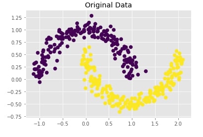
Create Moons Dataset (Two Interleaving Circles) 
Below we are creating two half interleaving circles using make_moons() method of scikit-learn's datasets module. It creates a dataset with 400 samples and 2 class labels.
We are also plotting the dataset to understand the dataset that was created.
X, Y = datasets.make_moons(n_samples=400,
                  noise=0.09,
                  random_state=1)

print('Dataset Size : ',X.shape, Y.shape)
with plt.style.context("ggplot"):
    plt.scatter(X[:,0],X[:,1], c = Y, marker="o", s=50)
    plt.title("Original Data");
Trying Agglomerative Clustering With Different Linkage 
We'll now try agglomerative clustering with different linkage algorithms on a dataset created above to check how each clustering algorithm is performing on it.
Agglomerative Clustering - Complete Linkage
clustering = AgglomerativeClustering(n_clusters=2, linkage="complete")
Y_preds = clustering.fit_predict(X)
Evaluating Performance Of Clustering Algorithm
adjusted_rand_score(Y, Y_preds)
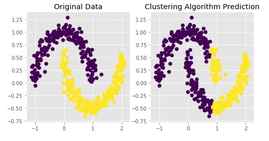
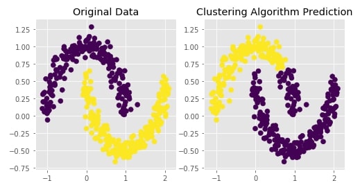
Visualizing Original and Predicted Labels for Comparison
def plot_actual_prediction_moons(X,Y,Y_preds):
    with plt.style.context("ggplot"):
        plt.figure(figsize=(8,4))

        plt.subplot(1,2,1)
        plt.scatter(X[:,0],X[:,1], c = Y, marker="o", s=50)
        plt.title("Original Data")

        plt.subplot(1,2,2)
        plt.scatter(X[:,0],X[:,1], c = Y_preds , marker="o", s=50)

        plt.title("Clustering Algorithm Prediction");

plot_actual_prediction_moons(X, Y, Y_preds)
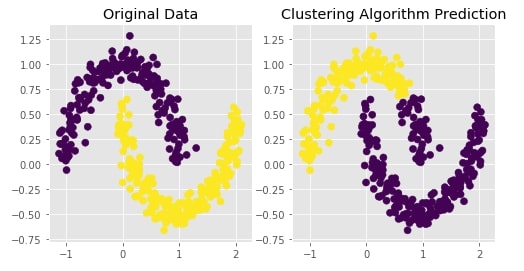
Agglomerative Clustering - Single Likage
clustering = AgglomerativeClustering(n_clusters=2, linkage="single")
Y_preds = clustering.fit_predict(X)
Evaluating Performance Of Clustering Algorithm
adjusted_rand_score(Y, Y_preds)
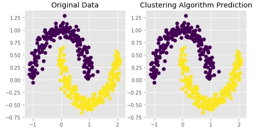
Visualizing Original and Predicted Labels for Comparison
plot_actual_prediction_moons(X, Y, Y_preds)
Agglomerative Clustering - Ward Linkage
clustering = AgglomerativeClustering(n_clusters=2, linkage="ward")
Y_preds = clustering.fit_predict(X)
Evaluating Performance Of Clustering Algorithm
adjusted_rand_score(Y, Y_preds)
Visualizing Original and Predicted Labels for Comparison
plot_actual_prediction_moons(X, Y, Y_preds)
Agglomerative Clustering - Average Linkage
clustering = AgglomerativeClustering(n_clusters=2, linkage="average")
Y_preds = clustering.fit_predict(X)
Evaluating Performance Of Clustering Algorithm
adjusted_rand_score(Y, Y_preds)
Visualizing Original and Predicted Labels for Comparison
plot_actual_prediction_moons(X, Y, Y_preds)
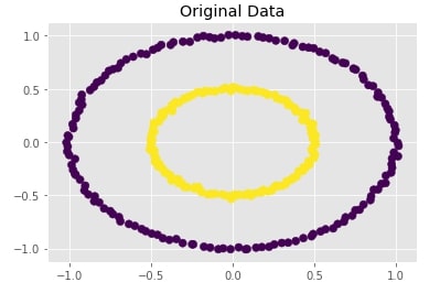
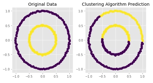
Create Dataset Of Circles (Large Circle Containing A Smaller Circle) 
Below we are creating a dataset which has one circle inside another circle. It creates a dataset with 300 samples and 2 class labels representing each circle.
We are also plotting the dataset to look at data.
from sklearn import datasets

X, Y  = datasets.make_circles(n_samples=300, noise=0.01,factor=0.5)
print('Dataset Size : ',X.shape, Y.shape)
with plt.style.context("ggplot"):
    plt.scatter(X[:,0],X[:,1], c = Y, marker="o", s=50)
    plt.title("Original Data");
Trying Agglomerative Clustering With Different Linkage 
We'll now try agglomerative clustering with different linkage algorithms on a dataset created above to check how each clustering algorithm is performing on it.
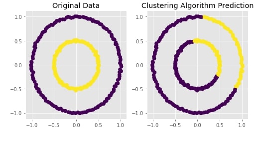
Agglomerative Clustering - Complete Linkage
clustering = AgglomerativeClustering(n_clusters=2, linkage="complete")
Y_preds = clustering.fit_predict(X)
Evaluating Performance Of Clustering Algorithm
adjusted_rand_score(Y, Y_preds)
Visualizing Original and Predicted Labels for Comparison
plot_actual_prediction_moons(X, Y, Y_preds)
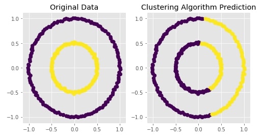
Agglomerative Clustering - Average Linkage
clustering = AgglomerativeClustering(n_clusters=2, linkage="average")
Y_preds = clustering.fit_predict(X)
Evaluating Performance Of Clustering Algorithm
adjusted_rand_score(Y, Y_preds)
Visualizing Original and Predicted Labels for Comparison
plot_actual_prediction_moons(X, Y, Y_preds)
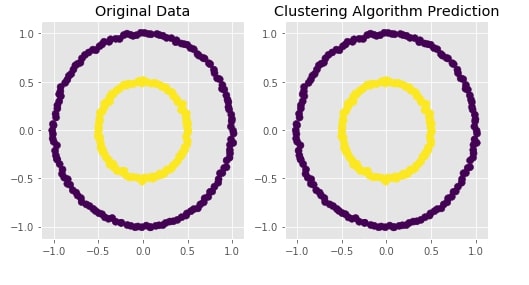
Agglomerative Clustering - Single Linkage
clustering = AgglomerativeClustering(n_clusters=2, linkage="single")
Y_preds = clustering.fit_predict(X)
Evaluating Performance Of Clustering Algorithm
adjusted_rand_score(Y, Y_preds)
Visualizing Original and Predicted Labels for Comparison
plot_actual_prediction_moons(X, Y, Y_preds)
Agglomerative Clustering - Ward
clustering = AgglomerativeClustering(n_clusters=2, linkage="ward")
Y_preds = clustering.fit_predict(X)
Evaluating Performance Of Clustering Algorithm
adjusted_rand_score(Y, Y_preds)
Visualizing Original and Predicted Labels for Comparison
plot_actual_prediction_moons(X, Y, Y_preds)
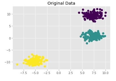
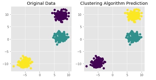
Create Isotropic Gaussian Blobs dataset 
Below we are creating isotropic Gaussian blobs dataset for clustering. It creates a dataset with 3 blobs. It has 400 samples and 3 class labels each representing blob label.
We are also plotting the dataset to understand it better.
X, Y = datasets.make_blobs(n_samples=400, random_state=8)

with plt.style.context("ggplot"):
    plt.scatter(X[:,0],X[:,1], c = Y, marker="o", s=50)
    plt.title("Original Data");
Trying Agglomerative Clustering With Different Linkage 
We'll now try agglomerative clustering with different linkage algorithms on a dataset created above to check how each clustering algorithm is performing on it.
Agglomerative Clustering - Ward
clustering = AgglomerativeClustering(n_clusters=3, linkage="ward")
Y_preds = clustering.fit_predict(X)
Evaluating Performance Of Clustering Algorithm
adjusted_rand_score(Y, Y_preds)
Visualizing Original and Predicted Labels for Comparison
plot_actual_prediction_moons(X, Y, Y_preds)
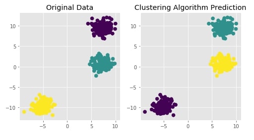
Agglomerative Clustering - Single Linkage
clustering = AgglomerativeClustering(n_clusters=3, linkage="single")
Y_preds = clustering.fit_predict(X)
Evaluating Performance Of Clustering Algorithm
adjusted_rand_score(Y, Y_preds)
Visualizing Original and Predicted Labels for Comparison
plot_actual_prediction_moons(X, Y, Y_preds)
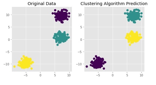
Agglomerative Clustering - Complete Linkage
clustering = AgglomerativeClustering(n_clusters=3, linkage="complete")
Y_preds = clustering.fit_predict(X)
Evaluating Performance Of Clustering Algorithm
adjusted_rand_score(Y, Y_preds)
Visualizing Original and Predicted Labels for Comparison
plot_actual_prediction_moons(X, Y, Y_preds)
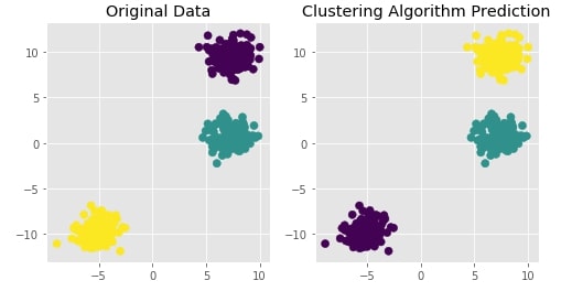
Agglomerative Clustering - Average Linkage
clustering = AgglomerativeClustering(n_clusters=3, linkage="average")
Y_preds = clustering.fit_predict(X)
Evaluating Performance Of Clustering Algorithm
adjusted_rand_score(Y, Y_preds)
Visualizing Original and Predicted Labels for Comparison
plot_actual_prediction_moons(X, Y, Y_preds)
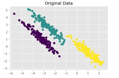
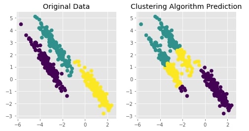
Create Isotropic Gaussian Blobs dataset & Skew Blobs Using Transformation 
Below we are again creating a Gaussian blobs dataset but this time we are also skewing blobs by adding noise data to it.
random_state = 170
X, Y = datasets.make_blobs(n_samples=400, random_state=random_state)
transformation = [[0.6, -0.6], [-0.4, 0.8]]
X = np.dot(X, transformation)
with plt.style.context("ggplot"):
    plt.scatter(X[:,0],X[:,1], c = Y, marker="o", s=50)
    plt.title("Original Data");
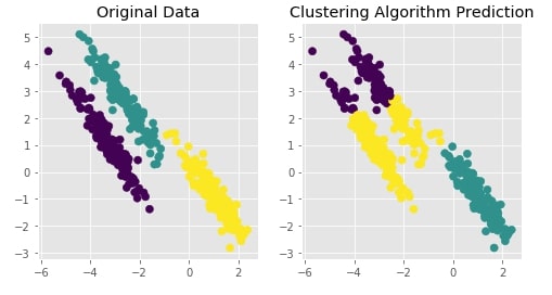
Trying Agglomerative Clustering With Different Linkage 
We'll now try agglomerative clustering with different linkage algorithms on a dataset created above to check how each clustering algorithm is performing on it.
Agglomerative Clustering - Average Linkage
clustering = AgglomerativeClustering(n_clusters=3, linkage="average")
Y_preds = clustering.fit_predict(X)
Evaluating Performance Of Clustering Algorithm
adjusted_rand_score(Y, Y_preds)
Visualizing Original and Predicted Labels for Comparison
plot_actual_prediction_moons(X, Y, Y_preds)
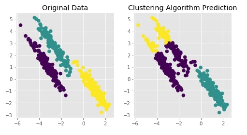
Agglomerative Clustering - Ward
clustering = AgglomerativeClustering(n_clusters=3, linkage="ward")
Y_preds = clustering.fit_predict(X)
Evaluating Performance Of Clustering Algorithm
adjusted_rand_score(Y, Y_preds)
Visualizing Original and Predicted Labels for Comparison
plot_actual_prediction_moons(X, Y, Y_preds)
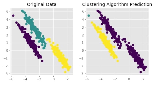
Agglomerative Clustering - Single Linkage
clustering = AgglomerativeClustering(n_clusters=3, linkage="single")
Y_preds = clustering.fit_predict(X)
Evaluating Performance Of Clustering Algorithm
adjusted_rand_score(Y, Y_preds)
Visualizing Original and Predicted Labels for Comparison
plot_actual_prediction_moons(X, Y, Y_preds)
Agglomerative Clustering - Complete Linkage
clustering = AgglomerativeClustering(n_clusters=3, linkage="complete")
Y_preds = clustering.fit_predict(X)
Evaluating Performance Of Clustering Algorithm
adjusted_rand_score(Y, Y_preds)
Visualizing Original and Predicted Labels for Comparison
plot_actual_prediction_moons(X, Y, Y_preds)
This ends our small tutorial explaining how to perform hierarchical clustering using scikit-learn. Please feel free to let us know your views in the comments section.
References 
 Sunny Solanki
Sunny Solanki
Intro: Software Developer | Youtuber | Bonsai Enthusiast
About: Sunny Solanki holds a bachelor's degree in Information Technology (2006-2010) from L.D. College of Engineering. Post completion of his graduation, he has 8.5+ years of experience (2011-2019) in the IT Industry (TCS). His IT experience involves working on Python & Java Projects with US/Canada banking clients. Since 2020, he’s primarily concentrating on growing CoderzColumn.
His main areas of interest are AI, Machine Learning, Data Visualization, and Concurrent Programming. He has good hands-on with Python and its ecosystem libraries.
Apart from his tech life, he prefers reading biographies and autobiographies. And yes, he spends his leisure time taking care of his plants and a few pre-Bonsai trees.
Contact: sunny.2309@yahoo.in


![YouTube Subscribe]() Comfortable Learning through Video Tutorials?
Comfortable Learning through Video Tutorials?
If you are more comfortable learning through video tutorials then we would recommend that you subscribe to our YouTube channel.
![Need Help]() Stuck Somewhere? Need Help with Coding? Have Doubts About the Topic/Code?
Stuck Somewhere? Need Help with Coding? Have Doubts About the Topic/Code?
 Stuck Somewhere? Need Help with Coding? Have Doubts About the Topic/Code?
When going through coding examples, it's quite common to have doubts and errors.
If you have doubts about some code examples or are stuck somewhere when trying our code, send us an email at coderzcolumn07@gmail.com. We'll help you or point you in the direction where you can find a solution to your problem.
You can even send us a mail if you are trying something new and need guidance regarding coding. We'll try to respond as soon as possible.
![Share Views]() Want to Share Your Views? Have Any Suggestions?
Want to Share Your Views? Have Any Suggestions?
 Want to Share Your Views? Have Any Suggestions?
If you want to
- provide some suggestions on topic
- share your views
- include some details in tutorial
- suggest some new topics on which we should create tutorials/blogs
 sklearn, hierarchical-clustering