Scikit-Learn - Clustering: Density-Based Clustering of Applications with Noise [DBSCAN]
Table of Contents
- Introduction
- Fitting DBSCAN on IRIS Data with Default Parameters
- Important Parameters of DBSCAN
- Create Moons Dataset (Two Interleaving Circles)
- Create Dataset Of Circles (Large Circle Containing A Smaller Circle)
- Create Isotropic Gaussian Blobs dataset & Skew Blobs Using Transformation
- References
Introduction 
DBSCAN stands for Density-based Spatial Clustering of Applications with Noise. One can sense from its name that, it divides the dataset into subgroup based on dense regions. DBSCAN does not require us to provide a number of clusters upfront.
The below image describes the concept of DBSCAN.
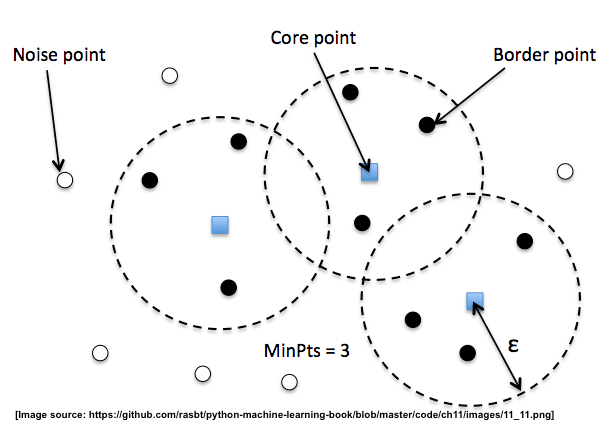
We define 3 different types of points for DBSCAN:
- Core Points: A core point is a point that has at least a minimum number of other points (
MinPts) in its radiusepsilon. - Border Points: A border point is a point that is not a core point, since it doesn't have enough
MinPtsin its neighborhood, but lies within the radius epsilon of a core point. - Noise Points: All other points that are neither core points nor border points.
The parameters like MinPoints and radius eps are commonly tuned in order to get the best results when using DBSCAN.
Scikit-Learn provides an implementation of DBSCAN as a part of the cluster module. We'll be explaining the usage of it as a part of this tutorial.
We'll start by importing the necessary libraries for our purpose.
import matplotlib.pyplot as plt
import numpy as np
import pandas as pd

import sklearn

%matplotlib inline
Load IRIS Data 
We'll load IRIS data for explanation purposes. It has a measurement of 3 different types of iris flowers. We'll use DBSCAN to group flowers of the same type into one cluster.
from sklearn import datasets

iris = datasets.load_iris()
X, Y = iris.data[:, [2,3]], iris.target

print("Features : ", iris.feature_names)
print("Target : ", iris.target_names)
print('Dataset Size : ', X.shape, Y.shape)
Below we have plotted dataset as scatter plot depicting sepal length versus sepal width relationship between each sample of data. We also have color-encoded points according to the flower category.
with plt.style.context("ggplot"):
    plt.scatter(X[:,0],X[:,1], c = Y, marker="o", s=50)
    plt.xlabel(iris.feature_names[0])
    plt.ylabel(iris.feature_names[1])
    plt.title("Original Data");
![Scikit-Learn - Clustering: Density-Based Clustering of Applications with Noise [DBSCAN]](/static/tutorials/machine_learning/dbscan-1.jpg)
We have designed a method named plot_actual_prediction_iris for plotting which can be used to compare original image labels and labels predicted by DBSCAN. It can help us analyze the performance of the DBSCAN algorithm. It accepts original data, labels, and predicted labels. It then plots original data color-encoded according to the original cluster label and original data color-encoded according to predicted(DBSCAN) cluster labels. We'll be using this method repetitively.
def plot_actual_prediction_iris(X, Y, Y_preds):
    with plt.style.context(("ggplot", "seaborn")):
        plt.figure(figsize=(17,6))

        plt.subplot(1,2,1)
        plt.scatter(X[Y==0,0],X[Y==0,1], c = 'red', marker="^", s=50)
        plt.scatter(X[Y==1,0],X[Y==1,1], c = 'green', marker="^", s=50)
        plt.scatter(X[Y==2,0],X[Y==2,1], c = 'blue', marker="^", s=50)
        plt.xlabel(iris.feature_names[0])
        plt.ylabel(iris.feature_names[1])
        plt.title("Original Data")

        plt.subplot(1,2,2)
        plt.scatter(X[Y_preds==0,0],X[Y_preds==0,1], c = 'red', marker="^", s=50)
        plt.scatter(X[Y_preds==1,0],X[Y_preds==1,1], c = 'green', marker="^", s=50)
        plt.scatter(X[Y_preds==2,0],X[Y_preds==2,1], c = 'blue', marker="^", s=50)
        plt.xlabel(iris.feature_names[0])
        plt.ylabel(iris.feature_names[1])
        plt.title("Clustering Algorithm Prediction");
Fitting DBSCAN on IRIS Data with Default Parameters 
from sklearn.cluster import DBSCAN

db = DBSCAN()

Y_preds = db.fit_predict(X)

Y_preds
Visualizing Clustering Results
plot_actual_prediction_iris(X, Y, Y_preds)
![Scikit-Learn - Clustering: Density-Based Clustering of Applications with Noise [DBSCAN]](/static/tutorials/machine_learning/dbscan-2.jpg)
Evaluating Performance of DBSCAN
We'll be using the adjusted_rand_score method for measuring the performance of the clustering algorithm by giving original labels and predicted labels as input to the method. It tries all possible pairs of clustering labels and returns a value between -1.0 and 1.0. If the clustering algorithm has predicted labels randomly then it'll return value of 0.0. If the value of 1.0 is returned then it means that the algorithm predicted all labels correctly.
from sklearn.metrics import adjusted_rand_score

adjusted_rand_score(Y, Y_preds)
Important Parameters of DBSCAN 
Below is a list of important parameters of DBSCAN which can be tuned to improve the performance of the clustering algorithm:
- eps - It accepts float value specifying the radius of the cluster as discussed above during introduction.
default=0.5 - min_samples - It accepts integer value specifying the number of neighboring samples to look to consider the sample as part of a particular cluster.
default=5 - metric - It accepts a string or callable specifying metric to use to calculate the distance between two points.
default=euclidean - algorithm - It accepts string value specifying the algorithm to use for nearest neighbors to point pointwise distances and find nearest neighbors. Below is a list of possible values.
auto- Default.ball_treekd_treebrute
- leaf_size - It accepts integer value specifying leaf size to pass to ball tree and kd tree algorithm.
db = DBSCAN(eps=0.2, min_samples=8, )

Y_preds = db.fit_predict(X)

Y_preds
Visualizing Clustering Results
plot_actual_prediction_iris(X, Y, Y_preds)
![Scikit-Learn - Clustering: Density-Based Clustering of Applications with Noise [DBSCAN]](/static/tutorials/machine_learning/dbscan-3.jpg)
Evaluating Performance of DBSCAN
adjusted_rand_score(Y, Y_preds)
Important Attributes of DBSCAN
Below is a list of important attributes of DBSCAN which can give meaningful insight once the model is trained:
core_sample_indices_- It returns an array of indices of core samples.components_- It returns an array of size (n_core_samples, n_features) specifying copy of each core sample found by training.
print("Size of Core Samples : ", db.core_sample_indices_.shape)

db.core_sample_indices_[:5]
print("Size of Components : ", db.components_.shape)
Create Moons Dataset (Two Interleaving Circles) 
Below we are creating two half interleaving circles using make_moons() method of scikit-learn's datasets module. It creates a dataset with 400 samples and 2 class labels.
We are also plotting the dataset to understand the dataset that was created.
X, Y = datasets.make_moons(n_samples=400,
                  noise=0.09,
                  random_state=1)
print('Dataset Size : ',X.shape, Y.shape)

with plt.style.context("ggplot"):
    plt.scatter(X[:,0],X[:,1], c = Y, marker="o", s=50)
    plt.title("Original Data");
![Scikit-Learn - Clustering: Density-Based Clustering of Applications with Noise [DBSCAN]](/static/tutorials/machine_learning/dbscan-4.jpg)
Trying Different Parameter Combination of DBSCAN on Data 
def plot_actual_prediction(X,Y,Y_preds):
    with plt.style.context("ggplot"):
        plt.figure(figsize=(6,3))

        plt.subplot(1,2,1)
        plt.scatter(X[:,0],X[:,1], c = Y, marker="o", s=50)
        plt.title("Original Data")

        plt.subplot(1,2,2)
        plt.scatter(X[:,0],X[:,1], c = Y_preds , marker="o", s=50)

        plt.title("Clustering Algorithm Prediction");

db = DBSCAN(eps=0.2,
            min_samples=5,
            metric='euclidean')
Y_preds = db.fit_predict(X)

plot_actual_prediction(X, Y, Y_preds)
![Scikit-Learn - Clustering: Density-Based Clustering of Applications with Noise [DBSCAN]](/static/tutorials/machine_learning/dbscan-5.jpg)
db = DBSCAN(eps=0.1,
            min_samples=5,
            metric='euclidean')
Y_preds = db.fit_predict(X)

plot_actual_prediction(X, Y, Y_preds)
![Scikit-Learn - Clustering: Density-Based Clustering of Applications with Noise [DBSCAN]](/static/tutorials/machine_learning/dbscan-6.jpg)
Create Dataset Of Circles (Large Circle Containing A Smaller Circle) 
Below we are creating a dataset that has one circle inside another circle. It creates a dataset with 300 samples and 2 class labels representing each circle.
We are also plotting the dataset to look at data.
X, Y  = datasets.make_circles(n_samples=300, noise=0.01,factor=0.5)
print('Dataset Size : ',X.shape, Y.shape)

with plt.style.context("ggplot"):
    plt.scatter(X[:,0],X[:,1], c = Y, marker="o", s=50)
    plt.title("Original Data");
![Scikit-Learn - Clustering: Density-Based Clustering of Applications with Noise [DBSCAN]](/static/tutorials/machine_learning/dbscan-7.jpg)
Trying Different Parameter Combination of DBSCAN on Data 
db = DBSCAN(eps=0.2,
            min_samples=15,
            metric='euclidean')
Y_preds = db.fit_predict(X)

plot_actual_prediction(X, Y, Y_preds)
![Scikit-Learn - Clustering: Density-Based Clustering of Applications with Noise [DBSCAN]](/static/tutorials/machine_learning/dbscan-8.jpg)
db = DBSCAN(eps=0.1,
            min_samples=7,
            metric='euclidean')
Y_preds = db.fit_predict(X)

plot_actual_prediction(X, Y, Y_preds)
![Scikit-Learn - Clustering: Density-Based Clustering of Applications with Noise [DBSCAN]](/static/tutorials/machine_learning/dbscan-9.jpg)
db = DBSCAN(eps=0.1,
            min_samples=15,
            metric='euclidean')
Y_preds = db.fit_predict(X)

plot_actual_prediction(X, Y, Y_preds)
![Scikit-Learn - Clustering: Density-Based Clustering of Applications with Noise [DBSCAN]](/static/tutorials/machine_learning/dbscan-10.jpg)
Create Isotropic Gaussian Blobs dataset & Skew Blobs Using Transformation 
Below we are creating isotropic Gaussian blobs dataset for clustering. It creates a dataset with 3 blobs. It has 400 samples and 3 class labels each representing blob label. We have also skewed blobs by adding noise data to it.
We are also plotting the dataset to understand it better.
random_state = 170
X, Y = datasets.make_blobs(n_samples=400, random_state=random_state)
transformation = [[0.6, -0.6], [-0.4, 0.8]]
X = np.dot(X, transformation)

with plt.style.context("ggplot"):
    plt.scatter(X[:,0],X[:,1], c = Y, marker="o", s=50)
    plt.title("Original Data");
![Scikit-Learn - Clustering: Density-Based Clustering of Applications with Noise [DBSCAN]](/static/tutorials/machine_learning/dbscan-11.jpg)
Trying Different Parameter Combination of DBSCAN on Data 
db = DBSCAN(eps=0.2,
            min_samples=15,
            metric='euclidean')
Y_preds = db.fit_predict(X)

plot_actual_prediction(X, Y, Y_preds)
![Scikit-Learn - Clustering: Density-Based Clustering of Applications with Noise [DBSCAN]](/static/tutorials/machine_learning/dbscan-12.jpg)
db = DBSCAN(eps=0.5,
            min_samples=5,
            metric='euclidean')
Y_preds = db.fit_predict(X)

plot_actual_prediction(X, Y, Y_preds)
![Scikit-Learn - Clustering: Density-Based Clustering of Applications with Noise [DBSCAN]](/static/tutorials/machine_learning/dbscan-13.jpg)
db = DBSCAN(eps=0.8,
            min_samples=10,
            metric='euclidean')
Y_preds = db.fit_predict(X)

plot_actual_prediction(X, Y, Y_preds)
![Scikit-Learn - Clustering: Density-Based Clustering of Applications with Noise [DBSCAN]](/static/tutorials/machine_learning/dbscan-14.jpg)
This ends our small tutorial on the DBSCAN algorithm for clustering. Please feel free to let us know your views in the comments section.
References 
 Sunny Solanki
Sunny Solanki
Intro: Software Developer | Youtuber | Bonsai Enthusiast
About: Sunny Solanki holds a bachelor's degree in Information Technology (2006-2010) from L.D. College of Engineering. Post completion of his graduation, he has 8.5+ years of experience (2011-2019) in the IT Industry (TCS). His IT experience involves working on Python & Java Projects with US/Canada banking clients. Since 2020, he’s primarily concentrating on growing CoderzColumn.
His main areas of interest are AI, Machine Learning, Data Visualization, and Concurrent Programming. He has good hands-on with Python and its ecosystem libraries.
Apart from his tech life, he prefers reading biographies and autobiographies. And yes, he spends his leisure time taking care of his plants and a few pre-Bonsai trees.
Contact: sunny.2309@yahoo.in


![YouTube Subscribe]() Comfortable Learning through Video Tutorials?
Comfortable Learning through Video Tutorials?
If you are more comfortable learning through video tutorials then we would recommend that you subscribe to our YouTube channel.
![Need Help]() Stuck Somewhere? Need Help with Coding? Have Doubts About the Topic/Code?
Stuck Somewhere? Need Help with Coding? Have Doubts About the Topic/Code?
 Stuck Somewhere? Need Help with Coding? Have Doubts About the Topic/Code?
When going through coding examples, it's quite common to have doubts and errors.
If you have doubts about some code examples or are stuck somewhere when trying our code, send us an email at coderzcolumn07@gmail.com. We'll help you or point you in the direction where you can find a solution to your problem.
You can even send us a mail if you are trying something new and need guidance regarding coding. We'll try to respond as soon as possible.
![Share Views]() Want to Share Your Views? Have Any Suggestions?
Want to Share Your Views? Have Any Suggestions?
 Want to Share Your Views? Have Any Suggestions?
If you want to
- provide some suggestions on topic
- share your views
- include some details in tutorial
- suggest some new topics on which we should create tutorials/blogs
 sklearn, dbscan, clustering