Updated On : Jun-07,2022 Time Investment : ~30 mins

Keras: RNNs (LSTM) for Text Generation (Character Embeddings)

Text Generation is an area of natural language processing (NLP) where we train models on the existing corpus of data and then generate new data. The models used for text generation tasks as generally referred to as language models. The language models are commonly used for tasks like conversational systems (chatbots), text summarization, text translation, etc. With the rise of deep learning, language models are created as deep neural networks. Recurrent neural networks (RNNs) are generally preferred to create language models for text generation tasks. The RNNs and their variants (LSTM, GRU, etc) are quite good at remembering sequences in data. They take into consideration previously seen examples to make predictions for the current. This approach makes them a better choice for text generation as we want the model to take into consideration previous words/characters when making predictions of the next word/character.

As a part of this tutorial, we have explained how to create Recurrent Neural Networks (RNNs) consisting of LSTM layers for text generation tasks using Python deep learning library Keras. We have used character-based approach for text generation where our model takes a specified number of words as input and predicts the next character that it thinks should come after them. To encode text data to real-valued data for the network, we have used word embeddings approach where we assign a real-valued vector of specified length to each unique character of the corpus. For training purposes, we have used Wikipedia article dataset available from torchtext library. We have another tutorial on text generation using Keras which does not use character embeddings and is based on only a bag of words. Please feel free to check it from the below link.

Below, we have listed important sections of tutorial to give an overview of the material covered in it.

Important Sections Of Tutorial

  1. Prepare Dataset
    • 1.1 Load Dataset
    • 1.2 Populate Vocabulary
    • 1.3 Organize Data
  2. Define Model
  3. Compile And Train Model
  4. Generate Text
  5. Train For More Epochs
  6. Generate Text
  7. Train Even More
  8. Generate Text
  9. Further Recommendations

Below, we have imported the necessary libraries that we have used in our tutorial and printed their versions as well.

import tensorflow

from tensorflow import keras

print("Keras Version : {}".format(keras.__version__))
Keras Version : 2.6.0
import torchtext

print("TorchText Version : {}".format(torchtext.__version__))
TorchText Version : 0.10.1
import gc

1. Prepare Dataset

In this section, we are preparing data to be given to the neural network for processing. As we said earlier, we'll use character-based approach for text generation which means that we'll give a specified number of characters to the neural network and make it predict the next character after them. We have decided that we'll give 100 characters sequence to network and make it predict the next character after them. For encoding characters, we'll use character embeddings approach. Below, we have listed steps in short that we'll follow to prepare data.

  1. Load data.
  2. Loop through each text example of data and prepare a vocabulary of unique characters. A vocabulary is a simple mapping from a character to an integer index. Each unique character is assigned an index starting from 0.
  3. Move window of size 100 through text example taking 100 characters as data features (X) next character after them as target value (Y). To explain with an example.
    • Characters 1-100 will be data features (X) and character 101 will be the target value (Y).
    • Move the window by one character.
    • Characters 2-101 will be data features (X) and character 102 will be target value (Y).
    • Move the window by one character.
    • Characters 3-102 will be data features (X) and character 103 will be target value (Y).
    • Move the window by one character.
    • ... and so on.
  4. Retrieve the index for characters present in data features (X) and target values (Y) from our populated vocabulary. This step will transform data from text to integer format.
  5. For each character index present in data features (X), retrieve embeddings of those characters.

In short, we'll first transform data from text to integer index and then retrieve embeddings for the characters using those indexes. Steps 1-4 will be performed in this section whereas steps will be implemented in the neural network as an embedding layer. We'll update those character embeddings during the training process so that they are learned. Steps will become more clear as we implement them below one by one.

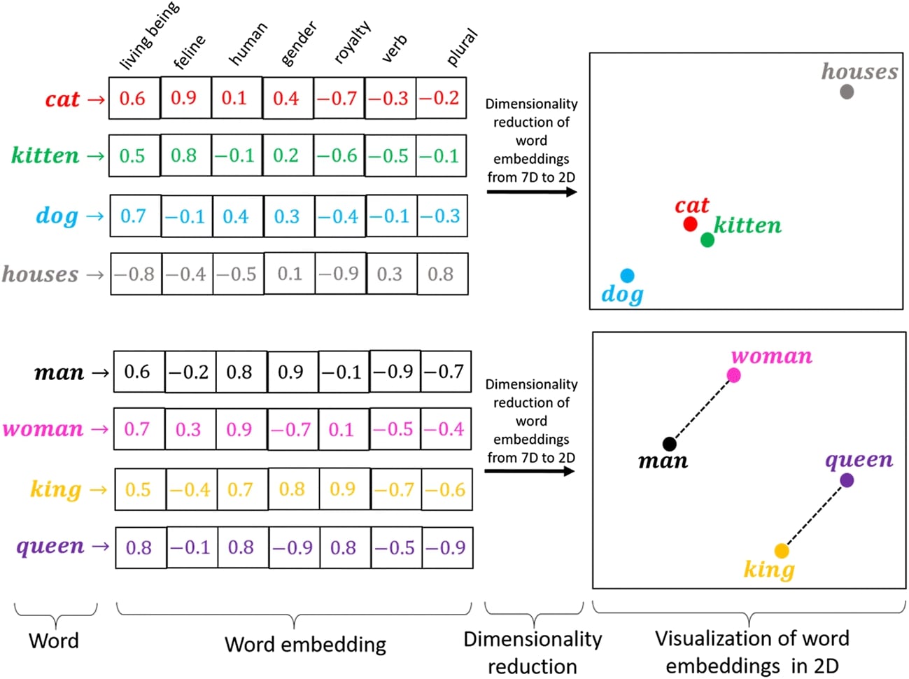
Below, we have included an image for word embeddings which is the same as character embeddings with the only difference being that words are considered tokens instead of characters. It'll give you an idea about embeddings. Embeddings give more representation power to tokens (character/n-gram/word).

Keras: Text Generation using Word Embeddings

1.1 Load Dataset

In this section, we have loaded Wikipedia dataset that we are going to use for our task. The dataset has a bunch of well-curated Wikipedia articles. The dataset is already divided into the train, validation, and test sets. We'll be using a training dataset for our case.

train_dataset, valid_dataset, test_dataset = torchtext.datasets.WikiText2()
wikitext-2-v1.zip: 100%|██████████| 4.48M/4.48M [00:00<00:00, 9.05MB/s]
X_train_text = [text for text in train_dataset]

len(X_train_text)
36718

1.2 Populate Vocabulary

In this section, we have populated the vocabulary of unique characters. In order to populate vocabulary, we have created an instance of Tokenizer available from preprocessing.text module of keras. We have set parameter char_level to True to inform the tokenizer to take characters as tokens. By default, it splits text into words. After defining the tokenizer, we have called fit_on_texts() method on the tokenizer with text examples to populate the vocabulary of unique characters. The vocabulary is available through word_index attribute of the tokenizer object.

After populating vocabulary, we have also printed it for reference purposes.

from keras.preprocessing.text import Tokenizer

tokenizer = Tokenizer(char_level=True)

tokenizer.fit_on_texts(X_train_text)
print(tokenizer.word_index)
{' ': 1, 'e': 2, 't': 3, 'a': 4, 'n': 5, 'i': 6, 'o': 7, 'r': 8, 's': 9, 'h': 10, 'd': 11, 'l': 12, 'u': 13, 'c': 14, 'm': 15, 'f': 16, 'g': 17, 'p': 18, 'w': 19, 'b': 20, 'y': 21, 'k': 22, ',': 23, '.': 24, 'v': 25, '<': 26, '>': 27, '@': 28, '\n': 29, '1': 30, '0': 31, '=': 32, '"': 33, '2': 34, "'": 35, '9': 36, '-': 37, 'j': 38, 'x': 39, ')': 40, '(': 41, '3': 42, '5': 43, '8': 44, '4': 45, '6': 46, '7': 47, 'z': 48, 'q': 49, ';': 50, '–': 51, ':': 52, '/': 53, '—': 54, '%': 55, 'é': 56, '$': 57, '[': 58, ']': 59, '&': 60, '!': 61, 'í': 62, '’': 63, 'á': 64, 'ā': 65, '£': 66, '°': 67, '?': 68, 'ó': 69, '+': 70, '#': 71, 'š': 72, '−': 73, 'ō': 74, 'ö': 75, 'è': 76, '×': 77, 'ü': 78, 'ä': 79, 'ʻ': 80, 'ś': 81, 'ć': 82, '“': 83, 'ø': 84, 'ł': 85, 'ç': 86, '”': 87, '₹': 88, 'ã': 89, 'µ': 90, 'ì': 91, 'ư': 92, '\ufeff': 93, 'æ': 94, '…': 95, '→': 96, 'ơ': 97, 'ñ': 98, 'å': 99, '☉': 100, '‘': 101, '~': 102, '*': 103, '⁄': 104, 'î': 105, '²': 106, 'ë': 107, 'ệ': 108, 'ī': 109, 'ú': 110, 'ễ': 111, 'ô': 112, 'à': 113, 'ū': 114, 'ă': 115, '^': 116, '♯': 117, 'ê': 118, '‑': 119, 'ỳ': 120, 'đ': 121, 'μ': 122, '≤': 123, 'ل': 124, '~': 125, 'ṃ': 126, '†': 127, '€': 128, '्': 129, '・': 130, '±': 131, 'ž': 132, 'ė': 133, '〈': 134, '〉': 135, 'β': 136, 'č': 137, 'α': 138, 'û': 139, '♭': 140, '½': 141, '„': 142, 'ị': 143, 'с': 144, 'ṭ': 145, 'γ': 146, 'â': 147, '′': 148, '大': 149, '空': 150, '̃': 151, 'ớ': 152, 'ầ': 153, '⅓': 154, 'ا': 155, 'ه': 156, 'ṅ': 157, '჻': 158, 'ṯ': 159, 'ş': 160, 'ح': 161, 'ص': 162, 'ن': 163, '″': 164, '³': 165, '¥': 166, '¡': 167, 'ấ': 168, 'ả': 169, '火': 170, '礮': 171, '·': 172, 'ḥ': 173, 'ჯ': 174, 'ი': 175, 'ო': 176, 'ხ': 177, 'ვ': 178, 'კ': 179, '戦': 180, '場': 181, 'の': 182, 'ヴ': 183, 'ァ': 184, 'ル': 185, 'キ': 186, 'ュ': 187, 'リ': 188, 'ア': 189, '₤': 190, 'ż': 191, 'ń': 192, '่': 193, 'ง': 194, 'ก': 195, 'ั': 196, 'ล': 197, 'ย': 198, 'า': 199, 'ณ': 200, 'ม': 201, 'ิ': 202, 'ต': 203, 'ร': 204, '์': 205, '§': 206, 'ス': 207, 'ト': 208, 'ッ': 209, 'プ': 210, 'ʿ': 211, 'þ': 212, '\\': 213, '`': 214, '⅔': 215, 'ắ': 216, 'ử': 217, '|': 218, '攻': 219, '殻': 220, '機': 221, '動': 222, '隊': 223, 'ų': 224, 'κ': 225, 'ò': 226, 'о': 227, 'в': 228, 'е': 229, 'т': 230, 'к': 231, 'а': 232, 'я': 233, 'ṣ': 234, 'დ': 235, 'უ': 236, 'ზ': 237, 'რ': 238, 'ს': 239, 'ძ': 240, 'წ': 241, 'გ': 242, 'ც': 243}

1.3 Organize Data

In this section, we are readying data for the network. The code loops through the sequence of text examples and move a window of 100 characters through them, adding 100 characters in data features (X_train) and a character after them in target values (Y_train).

Please make a NOTE that we have used fewer text examples for training purposes. The dataset has ~36k text examples and using all of them can take a lot of time.

After organizing data into data features (X_train) and target values (Y_train), we have retrieved the index of characters present in them using populated vocabulary. This index sequences now represents characters and will be given to the network for the training process.

Below, we have explained the data preparation process with a simple example.

vocab = {
'h':1,
'e':2,
'l':3,
'o':4,
' ':5,
',':6,
'w',7,
'a':8,
'r':9,
'y':10,
'u':11,
'?':12,
'c':13,
'm':14,
't':15,
'd':16,
'z':17,
'n':18
}

text_example = "Hello, How are you? Welcome to coderzcolumn?"
seq_length = 10

X_train = [
            ['h','e','l','l','o',',',' ', 'h','o','w'],
            [,'e','l','l','o',',',' ', 'h','o','w',' '],
            ['l','l','o',',',' ', 'h','o','w', ' ', 'a'],
            ['l','o',',',' ', 'h','o','w',' ', 'a', 'r'],
            ...
            ['d','e','r','z','c','o','l', 'u','m','n']
            ]
Y_train = ['e','l','l','o',',',' ', 'h','o','w',' ',..., '?']

X_train_vectorized = [
                        [1,2,3,4,5,6,1,4,7],
                        [2,3,4,5,6,1,4,7,5],
                        [3,4,5,6,1,4,7,5,1],
                        ...
                        [16,2,9,17,13,4,3,11,14,18]
                     ]
Y_train_vectorized = [1,2,3,4,5,6,1,4,7,5,1,...., 12]
%%time

import numpy as np
train_dataset, valid_dataset, test_dataset = torchtext.datasets.WikiText2()

seq_length = 100 ## Network Hyperparameter to tune
X_train, Y_train = [], []

for text in X_train_text[:6000]:## Using few text examples
    for i in range(0, len(text)-seq_length):
        inp_seq = text[i:i+seq_length].lower()
        out_seq = text[i+seq_length].lower()
        X_train.append(inp_seq)
        Y_train.append(tokenizer.word_index[out_seq]) ## Retrieve index for characters from vocabulary

X_train = tokenizer.texts_to_sequences(X_train) ## Retrieve index for characters from vocabulary

X_train, Y_train = np.array(X_train, dtype=np.int32), np.array(Y_train)

X_train.shape, Y_train.shape
CPU times: user 48.7 s, sys: 870 ms, total: 49.6 s
Wall time: 49.7 s
((1377719, 100), (1377719,))
gc.collect()
21

2. Define Model

In this section, we have defined a model that we'll use for our task. Our task will be considered a classification task as we are predicting one new character from a list of possible vocabulary characters. The network consists of 4 layers.

  1. Embedding Layer (Embedding Length = 50)
  2. LSTM Layer (Output Size = 256)
  3. LSTM Layer (Output Size = 256)
  4. Dense Layer (Output Units = vocab_size)

The first layer of the network is the embedding layer. We have created a layer using Embedding() constructor. We have provided vocabulary length as the input dimension and embedding length of 50 as the output dimension. This will create a weight matrix of shape (vocab_len, embed_len). This weight matrix has embeddings for each character of the vocabulary. We have already retrieved the index of characters from vocabulary which will be used to index this array to retrieve the embedding of characters. E.g, If index of character 'a' is 1 then weight_matrix[1] will return real-valued vector of shape (embed_len,) = (50,) representing embedding of character 'a'. The input shape to the layer is (batch_size, seq_length) and output data shape is (batch_size, seq_length, embed_len). This output will be given to the first LSTM layer for processing.

The first LSTM layer has 256 output units. It'll process the output of the embedding layer and output processed data of shape (batch_size, seq_length, 256). This output will be given to the second LSTM layer for the processing which will process it and output processed data of shape (batch_size, 256). The second LSTM layer does return the output of all processed sequences because we have not set return_sequences to True. It'll return an output of the last sequence (100th) for each example.

The output of the second LSTM layer is given to a dense layer for processing. The dense layer has the same output units as the length of vocabulary. The softmax activation function is applied to the output of the dense layer to convert them to probabilities.

After initializing the network, we have also printed a summary stating network layer output shapes and parameter counts.

Please make a NOTE that we have not covered embeddings and LSTM layer in deep here. If you are interested to learn about them then please check the below links. They cover topics in little detail for text classification tasks.

from tensorflow.keras.models import Sequential
from tensorflow.keras.layers import LSTM, Dense, Embedding

embed_len = 50
lstm_out = 256

model = Sequential([
                    Embedding(input_dim=len(tokenizer.word_index)+1, output_dim=embed_len,
                              input_length=seq_length),
                    LSTM(lstm_out, return_sequences=True),
                    LSTM(lstm_out),
                    Dense(len(tokenizer.word_index)+1, activation="softmax")
                ])


model.summary()
2022-05-29 04:15:35.381708: I tensorflow/stream_executor/cuda/cuda_gpu_executor.cc:937] successful NUMA node read from SysFS had negative value (-1), but there must be at least one NUMA node, so returning NUMA node zero
2022-05-29 04:15:35.382816: I tensorflow/stream_executor/cuda/cuda_gpu_executor.cc:937] successful NUMA node read from SysFS had negative value (-1), but there must be at least one NUMA node, so returning NUMA node zero
2022-05-29 04:15:35.383479: I tensorflow/stream_executor/cuda/cuda_gpu_executor.cc:937] successful NUMA node read from SysFS had negative value (-1), but there must be at least one NUMA node, so returning NUMA node zero
2022-05-29 04:15:35.384334: I tensorflow/core/platform/cpu_feature_guard.cc:142] This TensorFlow binary is optimized with oneAPI Deep Neural Network Library (oneDNN) to use the following CPU instructions in performance-critical operations:  AVX2 AVX512F FMA
To enable them in other operations, rebuild TensorFlow with the appropriate compiler flags.
2022-05-29 04:15:35.384604: I tensorflow/stream_executor/cuda/cuda_gpu_executor.cc:937] successful NUMA node read from SysFS had negative value (-1), but there must be at least one NUMA node, so returning NUMA node zero
2022-05-29 04:15:35.385295: I tensorflow/stream_executor/cuda/cuda_gpu_executor.cc:937] successful NUMA node read from SysFS had negative value (-1), but there must be at least one NUMA node, so returning NUMA node zero
2022-05-29 04:15:35.385999: I tensorflow/stream_executor/cuda/cuda_gpu_executor.cc:937] successful NUMA node read from SysFS had negative value (-1), but there must be at least one NUMA node, so returning NUMA node zero
2022-05-29 04:15:39.920872: I tensorflow/stream_executor/cuda/cuda_gpu_executor.cc:937] successful NUMA node read from SysFS had negative value (-1), but there must be at least one NUMA node, so returning NUMA node zero
2022-05-29 04:15:39.921695: I tensorflow/stream_executor/cuda/cuda_gpu_executor.cc:937] successful NUMA node read from SysFS had negative value (-1), but there must be at least one NUMA node, so returning NUMA node zero
2022-05-29 04:15:39.922348: I tensorflow/stream_executor/cuda/cuda_gpu_executor.cc:937] successful NUMA node read from SysFS had negative value (-1), but there must be at least one NUMA node, so returning NUMA node zero
2022-05-29 04:15:39.923570: I tensorflow/core/common_runtime/gpu/gpu_device.cc:1510] Created device /job:localhost/replica:0/task:0/device:GPU:0 with 14969 MB memory:  -> device: 0, name: Tesla P100-PCIE-16GB, pci bus id: 0000:00:04.0, compute capability: 6.0
Model: "sequential"
_________________________________________________________________
Layer (type)                 Output Shape              Param #
=================================================================
embedding (Embedding)        (None, 100, 50)           12200
_________________________________________________________________
lstm (LSTM)                  (None, 100, 256)          314368
_________________________________________________________________
lstm_1 (LSTM)                (None, 256)               525312
_________________________________________________________________
dense (Dense)                (None, 244)               62708
=================================================================
Total params: 914,588
Trainable params: 914,588
Non-trainable params: 0
_________________________________________________________________

3. Compile And Train Model

Here, we have first compiled our network to use Adam optimizer and cross entropy loss. After compiling the network, we have trained it for 50 epochs. We have used a batch size of 1024 during training. We can notice from the loss value getting printed after each epoch that our network seems to be doing a good job at the task.

from tensorflow.keras.optimizers import Adam
from keras import backend as K

model.compile(optimizer=Adam(learning_rate=0.001), loss="sparse_categorical_crossentropy")
model.fit(X_train, Y_train, batch_size=1024, epochs=50)
2022-05-29 04:15:41.569483: I tensorflow/compiler/mlir/mlir_graph_optimization_pass.cc:185] None of the MLIR Optimization Passes are enabled (registered 2)
Epoch 1/50
2022-05-29 04:15:44.812676: I tensorflow/stream_executor/cuda/cuda_dnn.cc:369] Loaded cuDNN version 8005
1346/1346 [==============================] - 160s 115ms/step - loss: 2.4106
Epoch 2/50
1346/1346 [==============================] - 156s 116ms/step - loss: 1.8968
Epoch 3/50
1346/1346 [==============================] - 156s 116ms/step - loss: 1.7443
Epoch 4/50
1346/1346 [==============================] - 156s 116ms/step - loss: 1.7566
Epoch 5/50
1346/1346 [==============================] - 156s 116ms/step - loss: 1.6260
Epoch 6/50
1346/1346 [==============================] - 156s 116ms/step - loss: 1.5180
Epoch 7/50
1346/1346 [==============================] - 156s 116ms/step - loss: 1.4932
Epoch 8/50
1346/1346 [==============================] - 156s 116ms/step - loss: 1.4591
Epoch 9/50
1346/1346 [==============================] - 156s 116ms/step - loss: 1.4312
Epoch 10/50
1346/1346 [==============================] - 156s 116ms/step - loss: 1.4032
Epoch 11/50
1346/1346 [==============================] - 156s 116ms/step - loss: 1.3758
Epoch 12/50
1346/1346 [==============================] - 156s 116ms/step - loss: 1.3558
Epoch 13/50
1346/1346 [==============================] - 156s 116ms/step - loss: 1.3383
Epoch 14/50
1346/1346 [==============================] - 156s 116ms/step - loss: 1.3262
Epoch 15/50
1346/1346 [==============================] - 156s 116ms/step - loss: 1.3170
Epoch 16/50
1346/1346 [==============================] - 156s 116ms/step - loss: 1.3072
Epoch 17/50
1346/1346 [==============================] - 156s 116ms/step - loss: 1.2951
Epoch 18/50
1346/1346 [==============================] - 156s 116ms/step - loss: 1.2997
Epoch 19/50
1346/1346 [==============================] - 156s 116ms/step - loss: 1.3036
Epoch 20/50
1346/1346 [==============================] - 156s 116ms/step - loss: 1.2839
Epoch 21/50
1346/1346 [==============================] - 156s 116ms/step - loss: 1.2697
Epoch 22/50
1346/1346 [==============================] - 156s 116ms/step - loss: 1.2602
Epoch 23/50
1346/1346 [==============================] - 156s 116ms/step - loss: 1.2463
Epoch 24/50
1346/1346 [==============================] - 157s 116ms/step - loss: 1.2498
Epoch 25/50
1346/1346 [==============================] - 156s 116ms/step - loss: 1.2071
Epoch 26/50
1346/1346 [==============================] - 156s 116ms/step - loss: 1.2329
Epoch 27/50
1346/1346 [==============================] - 157s 116ms/step - loss: 1.1923
Epoch 28/50
1346/1346 [==============================] - 157s 116ms/step - loss: 1.1788
Epoch 29/50
1346/1346 [==============================] - 157s 116ms/step - loss: 1.1648
Epoch 30/50
1346/1346 [==============================] - 157s 116ms/step - loss: 1.2089
Epoch 31/50
1346/1346 [==============================] - 157s 117ms/step - loss: 1.1933
Epoch 32/50
1346/1346 [==============================] - 156s 116ms/step - loss: 1.1812
Epoch 33/50
1346/1346 [==============================] - 156s 116ms/step - loss: 1.1645
Epoch 34/50
1346/1346 [==============================] - 157s 116ms/step - loss: 1.1523
Epoch 35/50
1346/1346 [==============================] - 157s 116ms/step - loss: 1.1427
Epoch 36/50
1346/1346 [==============================] - 157s 117ms/step - loss: 1.1363
Epoch 37/50
1346/1346 [==============================] - 157s 117ms/step - loss: 1.1298
Epoch 38/50
1346/1346 [==============================] - 157s 116ms/step - loss: 1.1235
Epoch 39/50
1346/1346 [==============================] - 157s 116ms/step - loss: 1.1185
Epoch 40/50
1346/1346 [==============================] - 157s 117ms/step - loss: 1.1121
Epoch 41/50
1346/1346 [==============================] - 157s 117ms/step - loss: 1.1039
Epoch 42/50
1346/1346 [==============================] - 157s 117ms/step - loss: 1.1040
Epoch 43/50
1346/1346 [==============================] - 156s 116ms/step - loss: 1.1153
Epoch 44/50
1346/1346 [==============================] - 156s 116ms/step - loss: 1.1146
Epoch 45/50
1346/1346 [==============================] - 156s 116ms/step - loss: 1.1057
Epoch 46/50
1346/1346 [==============================] - 157s 116ms/step - loss: 1.0944
Epoch 47/50
1346/1346 [==============================] - 157s 117ms/step - loss: 1.0870
Epoch 48/50
1346/1346 [==============================] - 157s 117ms/step - loss: 1.0798
Epoch 49/50
1346/1346 [==============================] - 157s 117ms/step - loss: 1.0757
Epoch 50/50
1346/1346 [==============================] - 156s 116ms/step - loss: 1.0725
<keras.callbacks.History at 0x7f5af0098190>

4. Generate Text

In this section, we are generating new text using our trained network. We are starting with randomly selecting an example from our dataset. After selecting an example, we have also printed the characters of the example. Then, we executed a loop 100 times to generate 100 new characters. The first iteration of the loop will start with characters of a randomly selected example. It'll then generate a new character, add it at the end of the selected example and remove the first character from the example to keep the length of sequence 100 characters. This process will be repeated for all iterations where we add a new character at the end and remove an existing first character. After generating 100 new characters, we have also printed them.

We can notice from the results that the network is able to spell words correctly and is also forming sentences. It is also generating punctuation marks. Though the sentences generated does not make much sense but it looks like English language sentence.

import random

random.seed(123)
idx = random.randint(0, len(X_train))
pattern = X_train[idx].flatten().tolist()

print("Initial Pattern : {}".format("".join([tokenizer.index_word[idx] for idx in pattern])))

generated_text = []
for i in range(100):
    X_batch = np.array(pattern, dtype=np.int32).reshape(1, seq_length) ## Design Batch
    preds = model.predict(X_batch) ## Make Prediction
    predicted_index = preds.argmax(axis=-1)[0] ## Retrieve token index
    generated_text.append(predicted_index) ## Add token index to result
    pattern.append(predicted_index) ## Add token index to original pattern
    pattern = pattern[1:] ## Resize pattern to bring again to seq_length length.

print("Generated Text : {}".format("".join([tokenizer.index_word[idx] for idx in generated_text])))
Initial Pattern : 1987 – 88 season where he was named the ihl 's co @-@ rookie of the year and most valuable player af
Generated Text : ter the second basketball operations of the second best @-@ searching the second basketball . the co

5. Train For More Epochs

In this section, we are training the network for another 50 epochs. We have set the learning rate to 0.0003 for training epochs. We can notice from the loss value getting printed after epochs that the network seems to be improving further.

K.set_value(model.optimizer.learning_rate, 0.0003)

model.fit(X_train, Y_train, batch_size=1024, epochs=50)
Epoch 1/50
1346/1346 [==============================] - 156s 116ms/step - loss: 1.0268
Epoch 2/50
1346/1346 [==============================] - 156s 116ms/step - loss: 1.0172
Epoch 3/50
1346/1346 [==============================] - 156s 116ms/step - loss: 1.0120
Epoch 4/50
1346/1346 [==============================] - 156s 116ms/step - loss: 1.0068
Epoch 5/50
1346/1346 [==============================] - 156s 116ms/step - loss: 1.0024
Epoch 6/50
1346/1346 [==============================] - 156s 116ms/step - loss: 0.9989
Epoch 7/50
1346/1346 [==============================] - 156s 116ms/step - loss: 0.9951
Epoch 8/50
1346/1346 [==============================] - 156s 116ms/step - loss: 0.9951
Epoch 9/50
1346/1346 [==============================] - 156s 116ms/step - loss: 0.9895
Epoch 10/50
1346/1346 [==============================] - 156s 116ms/step - loss: 0.9856
Epoch 11/50
1346/1346 [==============================] - 156s 116ms/step - loss: 0.9841
Epoch 12/50
1346/1346 [==============================] - 156s 116ms/step - loss: 0.9802
Epoch 13/50
1346/1346 [==============================] - 156s 116ms/step - loss: 0.9776
Epoch 14/50
1346/1346 [==============================] - 156s 116ms/step - loss: 0.9750
Epoch 15/50
1346/1346 [==============================] - 156s 116ms/step - loss: 0.9729
Epoch 16/50
1346/1346 [==============================] - 156s 116ms/step - loss: 0.9702
Epoch 17/50
1346/1346 [==============================] - 156s 116ms/step - loss: 0.9683
Epoch 18/50
1346/1346 [==============================] - 156s 116ms/step - loss: 0.9652
Epoch 19/50
1346/1346 [==============================] - 156s 116ms/step - loss: 0.9621
Epoch 20/50
1346/1346 [==============================] - 156s 116ms/step - loss: 0.9616
Epoch 21/50
1346/1346 [==============================] - 156s 116ms/step - loss: 0.9569
Epoch 22/50
1346/1346 [==============================] - 156s 116ms/step - loss: 0.9531
Epoch 23/50
1346/1346 [==============================] - 156s 116ms/step - loss: 0.9497
Epoch 24/50
1346/1346 [==============================] - 156s 116ms/step - loss: 0.9470
Epoch 25/50
1346/1346 [==============================] - 156s 116ms/step - loss: 0.9444
Epoch 26/50
1346/1346 [==============================] - 156s 116ms/step - loss: 0.9421
Epoch 27/50
1346/1346 [==============================] - 156s 116ms/step - loss: 0.9389
Epoch 28/50
1346/1346 [==============================] - 156s 116ms/step - loss: 0.9361
Epoch 29/50
1346/1346 [==============================] - 156s 116ms/step - loss: 0.9344
Epoch 30/50
1346/1346 [==============================] - 156s 116ms/step - loss: 0.9319
Epoch 31/50
1346/1346 [==============================] - 156s 116ms/step - loss: 0.9286
Epoch 32/50
1346/1346 [==============================] - 156s 116ms/step - loss: 0.9261
Epoch 33/50
1346/1346 [==============================] - 156s 116ms/step - loss: 0.9232
Epoch 34/50
1346/1346 [==============================] - 156s 116ms/step - loss: 0.9214
Epoch 35/50
1346/1346 [==============================] - 156s 116ms/step - loss: 0.9185
Epoch 36/50
1346/1346 [==============================] - 156s 116ms/step - loss: 0.9159
Epoch 37/50
1346/1346 [==============================] - 156s 116ms/step - loss: 0.9155
Epoch 38/50
1346/1346 [==============================] - 155s 115ms/step - loss: 0.9130
Epoch 39/50
1346/1346 [==============================] - 157s 116ms/step - loss: 0.9099
Epoch 40/50
1346/1346 [==============================] - 157s 116ms/step - loss: 0.9079
Epoch 41/50
1346/1346 [==============================] - 156s 116ms/step - loss: 0.9043
Epoch 42/50
1346/1346 [==============================] - 156s 116ms/step - loss: 0.9022
Epoch 43/50
1346/1346 [==============================] - 156s 116ms/step - loss: 0.8998
Epoch 44/50
1346/1346 [==============================] - 156s 116ms/step - loss: 0.8965
Epoch 45/50
1346/1346 [==============================] - 156s 116ms/step - loss: 0.8942
Epoch 46/50
1346/1346 [==============================] - 157s 117ms/step - loss: 0.8915
Epoch 47/50
1346/1346 [==============================] - 157s 117ms/step - loss: 0.8894
Epoch 48/50
1346/1346 [==============================] - 157s 117ms/step - loss: 0.8875
Epoch 49/50
1346/1346 [==============================] - 158s 117ms/step - loss: 0.8838
Epoch 50/50
1346/1346 [==============================] - 158s 117ms/step - loss: 0.8831
<keras.callbacks.History at 0x7f5ae86ab350>

6. Generate Text

In this section, we have again generated 100 new characters using our more trained network. Our network is now trained for a total of 100 epochs. We have started with the same example that we used earlier. We can notice from the results that our network is generating new words this time. Though it seems to be repeating some words. We'll train it further for more epochs to see whether it helps improve further.

import random

random.seed(123)
idx = random.randint(0, len(X_train))
pattern = X_train[idx].flatten().tolist()

print("Initial Pattern : {}".format("".join([tokenizer.index_word[idx] for idx in pattern])))

generated_text = []
for i in range(100):
    X_batch = np.array(pattern, dtype=np.int32).reshape(1, seq_length) ## Design Batch
    preds = model.predict(X_batch) ## Make Prediction
    predicted_index = preds.argmax(axis=-1)[0] ## Retrieve token index
    generated_text.append(predicted_index) ## Add token index to result
    pattern.append(predicted_index) ## Add token index to original pattern
    pattern = pattern[1:] ## Resize pattern to bring again to seq_length length.

print("Generated Text : {}".format("".join([tokenizer.index_word[idx] for idx in generated_text])))
Initial Pattern : 1987 – 88 season where he was named the ihl 's co @-@ rookie of the year and most valuable player af
Generated Text : ter a strong deported the conference finals . the second single , such as the second single in the s

7. Train Even More

In this section, we have reduced the learning rate to 0.0001 and trained the network for another 50 epochs. We can notice that loss is reducing further after each epoch which hints that the network is improving further.

K.set_value(model.optimizer.learning_rate, 0.0001)

model.fit(X_train, Y_train, batch_size=1024, epochs=50)
Epoch 1/50
1346/1346 [==============================] - 157s 117ms/step - loss: 0.8573
Epoch 2/50
1346/1346 [==============================] - 157s 116ms/step - loss: 0.8540
Epoch 3/50
1346/1346 [==============================] - 157s 117ms/step - loss: 0.8525
Epoch 4/50
1346/1346 [==============================] - 158s 117ms/step - loss: 0.8510
Epoch 5/50
1346/1346 [==============================] - 157s 117ms/step - loss: 0.8494
Epoch 6/50
1346/1346 [==============================] - 157s 117ms/step - loss: 0.8483
Epoch 7/50
1346/1346 [==============================] - 158s 117ms/step - loss: 0.8472
Epoch 8/50
1346/1346 [==============================] - 157s 117ms/step - loss: 0.8461
Epoch 9/50
1346/1346 [==============================] - 157s 117ms/step - loss: 0.8447
Epoch 10/50
1346/1346 [==============================] - 157s 117ms/step - loss: 0.8436
Epoch 11/50
1346/1346 [==============================] - 158s 117ms/step - loss: 0.8427
Epoch 12/50
1346/1346 [==============================] - 157s 117ms/step - loss: 0.8417
Epoch 13/50
1346/1346 [==============================] - 157s 117ms/step - loss: 0.8406
Epoch 14/50
1346/1346 [==============================] - 157s 117ms/step - loss: 0.8396
Epoch 15/50
1346/1346 [==============================] - 157s 117ms/step - loss: 0.8385
Epoch 16/50
1346/1346 [==============================] - 157s 117ms/step - loss: 0.8374
Epoch 17/50
1346/1346 [==============================] - 156s 116ms/step - loss: 0.8362
Epoch 18/50
1346/1346 [==============================] - 157s 117ms/step - loss: 0.8351
Epoch 19/50
1346/1346 [==============================] - 157s 117ms/step - loss: 0.8342
Epoch 20/50
1346/1346 [==============================] - 157s 117ms/step - loss: 0.8327
Epoch 21/50
1346/1346 [==============================] - 157s 117ms/step - loss: 0.8318
Epoch 22/50
1346/1346 [==============================] - 157s 117ms/step - loss: 0.8307
Epoch 23/50
1346/1346 [==============================] - 157s 117ms/step - loss: 0.8298
Epoch 24/50
1346/1346 [==============================] - 157s 117ms/step - loss: 0.8288
Epoch 25/50
1346/1346 [==============================] - 157s 117ms/step - loss: 0.8277
Epoch 26/50
1346/1346 [==============================] - 157s 117ms/step - loss: 0.8267
Epoch 27/50
1346/1346 [==============================] - 157s 117ms/step - loss: 0.8257
Epoch 28/50
1346/1346 [==============================] - 157s 117ms/step - loss: 0.8251
Epoch 29/50
1346/1346 [==============================] - 157s 117ms/step - loss: 0.8229
Epoch 30/50
1346/1346 [==============================] - 157s 117ms/step - loss: 0.8219
Epoch 31/50
1346/1346 [==============================] - 157s 117ms/step - loss: 0.8213
Epoch 32/50
1346/1346 [==============================] - 157s 117ms/step - loss: 0.8207
Epoch 33/50
1346/1346 [==============================] - 157s 117ms/step - loss: 0.8196
Epoch 34/50
1346/1346 [==============================] - 157s 117ms/step - loss: 0.8187
Epoch 35/50
1346/1346 [==============================] - 157s 117ms/step - loss: 0.8180
Epoch 36/50
1346/1346 [==============================] - 158s 117ms/step - loss: 0.8170
Epoch 37/50
1346/1346 [==============================] - 157s 117ms/step - loss: 0.8160
Epoch 38/50
1346/1346 [==============================] - 157s 117ms/step - loss: 0.8151
Epoch 39/50
1346/1346 [==============================] - 158s 117ms/step - loss: 0.8139
Epoch 40/50
1346/1346 [==============================] - 158s 117ms/step - loss: 0.8130
Epoch 41/50
1346/1346 [==============================] - 157s 117ms/step - loss: 0.8123
Epoch 42/50
1346/1346 [==============================] - 158s 117ms/step - loss: 0.8110
Epoch 43/50
1346/1346 [==============================] - 158s 117ms/step - loss: 0.8105
Epoch 44/50
1346/1346 [==============================] - 157s 117ms/step - loss: 0.8090
Epoch 45/50
1346/1346 [==============================] - 157s 117ms/step - loss: 0.8079
Epoch 46/50
1346/1346 [==============================] - 157s 117ms/step - loss: 0.8072
Epoch 47/50
1346/1346 [==============================] - 158s 117ms/step - loss: 0.8065
Epoch 48/50
1346/1346 [==============================] - 157s 117ms/step - loss: 0.8056
Epoch 49/50
1346/1346 [==============================] - 157s 117ms/step - loss: 0.8046
Epoch 50/50
1346/1346 [==============================] - 157s 117ms/step - loss: 0.8046
<keras.callbacks.History at 0x7f5af0196d50>

8. Generate Text

In this section, we have again generated new 100 characters using our trained network. We can notice from the results that the network is able to generate English words correctly. It has generated a new-line character as well this time. Next, we'll give some suggestions on how to improve network performance further.

import random

random.seed(123)
idx = random.randint(0, len(X_train))
pattern = X_train[idx].flatten().tolist()

print("Initial Pattern : {}".format("".join([tokenizer.index_word[idx] for idx in pattern])))

generated_text = []
for i in range(100):
    X_batch = np.array(pattern, dtype=np.int32).reshape(1, seq_length) ## Design Batch
    preds = model.predict(X_batch) ## Make Prediction
    predicted_index = preds.argmax(axis=-1)[0] ## Retrieve token index
    generated_text.append(predicted_index) ## Add token index to result
    pattern.append(predicted_index) ## Add token index to original pattern
    pattern = pattern[1:] ## Resize pattern to bring again to seq_length length.

print("Generated Text : {}".format("".join([tokenizer.index_word[idx] for idx in generated_text])))
Initial Pattern : 1987 – 88 season where he was named the ihl 's co @-@ rookie of the year and most valuable player af
Generated Text : ter a star @-@ linked continues of several position .
orether and second section was completed in t

9. Further Recommendations

  1. Try training the network for more epochs.
  2. Try different embedding lengths. We tried embedding a length of 50.
  3. Try different sequence lengths. We tried a sequence of 100 characters.
  4. Try different LSTM layers. Please make a NOTE that adding more LSTM layers will increase training time a lot.
  5. Try different output sizes for LSTM layers.
  6. Try adding more dense layers after LSTM layers.
  7. Try n-gram/word based models instead of character-based.
  8. Try learning rate schedulers
  9. Try other RNN layers (Vanilla RNN, GRU, etc) for processing sequences.
  10. Add little randomness to the prediction of the next character. REFERENCE
Sunny Solanki  Sunny Solanki

YouTube Subscribe Comfortable Learning through Video Tutorials?

If you are more comfortable learning through video tutorials then we would recommend that you subscribe to our YouTube channel.

Need Help Stuck Somewhere? Need Help with Coding? Have Doubts About the Topic/Code?

When going through coding examples, it's quite common to have doubts and errors.

If you have doubts about some code examples or are stuck somewhere when trying our code, send us an email at coderzcolumn07@gmail.com. We'll help you or point you in the direction where you can find a solution to your problem.

You can even send us a mail if you are trying something new and need guidance regarding coding. We'll try to respond as soon as possible.

Share Views Want to Share Your Views? Have Any Suggestions?

If you want to

  • provide some suggestions on topic
  • share your views
  • include some details in tutorial
  • suggest some new topics on which we should create tutorials/blogs
Please feel free to contact us at coderzcolumn07@gmail.com. We appreciate and value your feedbacks. You can also support us with a small contribution by clicking DONATE.


Subscribe to Our YouTube Channel

YouTube SubScribe

Newsletter Subscription