PyTorch: Learning Rate Schedules
Learning rate is one of the most important parameters of training a neural network that can impact the results of the network. When training a network using optimizers like SGD, the learning rate generally stays constant and does not change throughout the training process. Research has shown that as we train for more epochs, decreasing the learning rate little can improve the performance of the network. It can give a little boost to performance. The learning rate can be reduced after each epoch or batch. This process of decreasing the learning rate over time during the training process is generally referred to as learning rate scheduling or learning rate annealing in the machine learning community. Over time, there are various approaches tried to decrease the learning rate.
As a part of this tutorial, we'll be discussing various learning rate schedules available from PyTorch. We have tried to cover the majority of schedules available from it. We have chosen the Fashion MNIST dataset for our tutorial and will be training a simple CNN on it. We'll train CNN with various learning rate schedules and compare their results. We have also created visualizations showing how the learning rate changes during the training process. We are assuming that the reader has little background on Pytorch. Please feel free to check the below tutorial if you want to learn about CNN creation using Pytorch.
PyTorch let us change the learning rate in two different ways during the training process.
- After completion of each batch.
- After completion of each epoch.
We can modify code based on our requirements on when we want to change the learning rate. It even let us use more than one learning rate scheduler together which can be executed one after another to modify the learning rate using different formulas. We have explained in one of our examples how we can combine multiple learning rate schedulers as well.
Below, we have listed important sections of tutorial to give an overview of the material covered.
Important Sections of Tutorial
- Load Fashion MNIST Data
- Define CNN
- Train Network
- Constant Learning Rate
- Step LR Scheduler
- MultiStep LR Scheduler
- Multiplicative LR Scheduler
- Lambda LR Scheduler
- Exponential LR Scheduler
- One Cycle LR Scheduler
- Cyclic LR Scheduler
- Cosine Annealing LR Scheduler
- Cosine Annealing With Warm Restarts Scheduler
- Reduce LR On Plateau Scheduler
- Combining Multiple Schedulers
- Final Test Set Accuracy Comparison of Various Schedulers
Below, we have imported PyTorch and printed the version that we have used in our tutorial.
import torch

print("Torch Version : {}".format(torch.__version__))
Load Data 
In this section, we have loaded the Fashion MNIST dataset available from keras. The data has grayscale images of shape (28,28) pixels for 10 different fashion items. The dataset is already divided into the train (60k images) and test (10k images) sets. The below table has a mapping from index value to category name of the images.
| Label | Description |
|---|---|
| 0 | T-shirt/top |
| 1 | Trouser |
| 2 | Pullover |
| 3 | Dress |
| 4 | Coat |
| 5 | Sandal |
| 6 | Shirt |
| 7 | Sneaker |
| 8 | Bag |
| 9 | Ankle boot |
The keras provides dataset as numpy arrays whereas PyTorch networks require tensors hence we have converted them to PyTorch tensors. Later on, we have also created Dataset and DataLoader objects from tensors. The data loader objects will let us loop through data during the training process easier. We have kept a batch size of 128 samples when creating loader objects for train and test datasets.
from tensorflow import keras
from sklearn.model_selection import train_test_split

(X_train, Y_train), (X_test, Y_test) = keras.datasets.fashion_mnist.load_data()

X_train, X_test, Y_train, Y_test = torch.tensor(X_train, dtype=torch.float32),\
                                   torch.tensor(X_test, dtype=torch.float32),\
                                   torch.tensor(Y_train, dtype=torch.long),\
                                   torch.tensor(Y_test, dtype=torch.long)

X_train, X_test = X_train.reshape(-1,1,28,28), X_test.reshape(-1,1,28,28)

X_train, X_test = X_train/255.0, X_test/255.0

classes =  Y_train.unique().tolist()
class_labels = ["T-shirt/top","Trouser","Pullover","Dress","Coat","Sandal","Shirt","Sneaker","Bag","Ankle boot"]
mapping = dict(zip(classes, class_labels))

X_train.shape, X_test.shape, Y_train.shape, Y_test.shape
from torch.utils.data import TensorDataset, DataLoader

train_dataset = TensorDataset(X_train, Y_train)
test_dataset  = TensorDataset(X_test , Y_test)

train_loader = DataLoader(train_dataset, batch_size=128, shuffle=True)
test_loader = DataLoader(test_dataset, batch_size=128, shuffle=True)
Define CNN 
In this section, we have defined our convolutional neural network using Pytorch. Our network consists of 3 convolution layers and one linear layer. The convolution layers have 32, 16, and 8 output filters respectively. The kernel size of filters used by all three convolution layers is (3,3). We have also applied relu activation function to the output of each convolution layer. The output of the third convolution layer is flattened and then given as input to the linear layer. The linear layer has 10 units which are the same as the number of target classes.
from torch import nn

class ConvNet(nn.Module):
    def __init__(self):
        super(ConvNet, self).__init__()
        self.seq = nn.Sequential(
            nn.Conv2d(in_channels=1, out_channels=32, kernel_size=(3,3), padding="same"),
            nn.ReLU(),

            nn.Conv2d(in_channels=32, out_channels=16, kernel_size=(3,3), padding="same"),
            nn.ReLU(),

            nn.Conv2d(in_channels=16, out_channels=8, kernel_size=(3,3), padding="same"),
            nn.ReLU(),

            nn.Flatten(),
            nn.Linear(8*28*28, len(classes)),
            #nn.Softmax(dim=1)
        )

    def forward(self, x_batch):
        preds = self.seq(x_batch)
        return preds
conv_net = ConvNet()

conv_net
preds = conv_net(X_train[:5])

preds.shape
1. Constant Learning Rate 
In this section, we are training our network with a constant learning rate. We'll be recording the accuracy of the model on test data with various learning rate schedules along with a constant learning rate for comparison purposes later.
Below, we have designed three functions that we'll use for training. There is one main training function that takes model, loss function, train loader, validation loader, and a number of epochs as input. It then executes the training loop number of epochs times. During each epoch, it performs a forward pass through the network to make predictions, calculate loss, calculate gradients, and update network parameters. It also records the loss of each batch and prints the average training loss after completion of each epoch. At the end of each epoch, it even calculates validation accuracy and validation loss using the other two helper functions defined in the below cell. The training function returns validation accuracy after completion of total training.
from sklearn.metrics import accuracy_score
from tqdm import tqdm

def CalcValLoss(model, loss_func, val_loader):
    with torch.no_grad(): ## Prevents calculation of gradients
        val_losses = []
        for X_batch, Y_batch in val_loader:
            preds = model(X_batch)
            loss = loss_func(preds, Y_batch)
            val_losses.append(loss)
        print("Valid CategoricalCrossEntropy : {:.3f}".format(torch.tensor(val_losses).mean()))

def MakePredictions(model, loader):
    preds, Y_shuffled = [], []
    for X_batch, Y_batch in loader:
        preds.append(model(X_batch))
        Y_shuffled.append(Y_batch)

    preds = torch.cat(preds).argmax(axis=-1)
    Y_shuffled = torch.cat(Y_shuffled)
    return Y_shuffled, preds

def TrainModelInBatchesV1(model, loss_func, optimizer, train_loader, val_loader, epochs=5):
    for i in range(epochs):
        losses = [] ## Record loss of each batch
        for X_batch, Y_batch in tqdm(train_loader):
            preds = model(X_batch) ## Make Predictions by forward pass through network

            loss = loss_func(preds, Y_batch) ## Calculate Loss
            losses.append(loss) ## Record Loss

            optimizer.zero_grad() ## Zero weights before calculating gradients
            loss.backward() ## Calculate Gradients
            optimizer.step() ## Update Weights

        print("Train CategoricalCrossEntropy : {:.3f}".format(torch.tensor(losses).mean()))
        CalcValLoss(model, loss_func, val_loader)

        Y_test_shuffled, test_preds = MakePredictions(model, val_loader)
        val_acc = accuracy_score(Y_test_shuffled, test_preds)
        print("Val  Accuracy : {:.3f}".format(val_acc))
    return val_acc
Below, we have initialized a dictionary named scheduler_val_accs that will hold the test accuracy of each learning rate schedule that we'll try. We'll also include constant learning rate results for comparison purposes.
In the next cell, we are actually training our network using the training function defined in the previous cell. We have initialized a number of epochs to 15 and the learning rate to 0.001. Followed by it, we have initialized our network, loss function, and optimizer. Then, we have called our training function with the necessary parameters to perform the training of the network. The function returns test accuracy which we have recorded in the dictionary. We are treating the test dataset as a validation dataset in our training process.
scheduler_val_accs = {}
from torch.optim import SGD, RMSprop, Adam

#torch.manual_seed(42) ##For reproducibility.This will make sure that same random weights are initialized each time.
epochs = 15
learning_rate = torch.tensor(1e-3) # 0.001

conv_net = ConvNet()
cross_entropy_loss = nn.CrossEntropyLoss()
optimizer = SGD(params=conv_net.parameters(), lr=learning_rate)

val_acc = TrainModelInBatchesV1(conv_net, cross_entropy_loss, optimizer, train_loader, test_loader,epochs)
scheduler_val_accs["Constant Learning Rate"] = val_acc
2. Step LR Scheduler 
In this section, we are using the step LR scheduler available from Pytorch to change the learning rate during the training process. We have explained how we can code so that we can change learning after each epoch as well as after each batch.
Below, we have modified our training function which we have defined earlier. We have added an extra parameter named schedulers which accepts a list of schedulers. After completion of each epoch, we loop through schedulers and call step() method on it which will change the learning rate of an optimizer. The rest of the code is the same as our previous training function.
from tqdm import tqdm

def TrainModelInBatchesV2(model, loss_func, optimizer, schedulers, train_loader, val_loader, epochs=5):
    for i in range(epochs):
        losses = [] ## Record loss of each batch
        for X_batch, Y_batch in tqdm(train_loader):
            preds = model(X_batch) ## Make Predictions by forward pass through network

            loss = loss_func(preds, Y_batch) ## Calculate Loss
            losses.append(loss) ## Record Loss

            optimizer.zero_grad() ## Zero weights before calculating gradients
            loss.backward() ## Calculate Gradients
            optimizer.step() ## Update Weights

        for scheduler in schedulers: ## Apply Schedulers after complete epoch
            scheduler.step()

        print("Train CategoricalCrossEntropy : {:.3f}".format(torch.tensor(losses).mean()))
        CalcValLoss(model, loss_func, val_loader)

        Y_test_shuffled, test_preds = MakePredictions(model, val_loader)
        val_acc = accuracy_score(Y_test_shuffled, test_preds)
        print("Val  Accuracy : {:.3f}".format(val_acc))
    return val_acc
Below, we have trained our network by giving a step lr learning rate scheduler. All other network parameters are almost the same as our previous constant learning rate example. We have created step LR scheduler using StepLR() constructor available from lr_scheduler sub-module of optim sub-module of PyTorch. Below are important parameters of StepLR() constructor.
- optimizer - We need to give optimizer instance first.
- step_size - This parameter accepts integer value specifying after how many steps we need to change the learning rate. The step can be epoch or batch.
- gamma - It accepts floating-point value specifying multiplicative factor of learning rate decay.
- verbose - It accepts boolean values specifying whether to display messages when the learning rate changes or not.
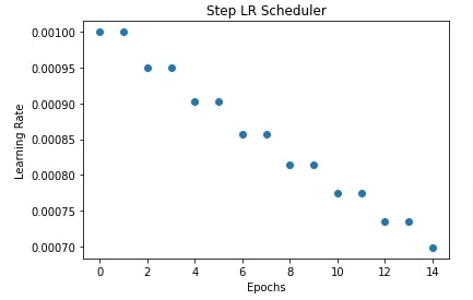
In our case, we are have initialized step lr scheduler with a step size of 2 hence it'll decrease the learning rate by a factor of 0.95 after every 2 epochs.
In the next cell after the training cell below, we have also collected values of learning rate after each epoch and plotted them to show how step LR scheduler changes learning rate internally.
from torch.optim import SGD, RMSprop, Adam
from torch.optim import lr_scheduler

#torch.manual_seed(42) ##For reproducibility.This will make sure that same random weights are initialized each time.
epochs = 15
learning_rate = torch.tensor(1e-3) # 0.001

conv_net = ConvNet()
cross_entropy_loss = nn.CrossEntropyLoss()
optimizer = SGD(params=conv_net.parameters(), lr=learning_rate)
scheduler = lr_scheduler.StepLR(optimizer, step_size=2, gamma=0.95, verbose=True)

val_acc = TrainModelInBatchesV2(conv_net, cross_entropy_loss, optimizer, [scheduler], train_loader, test_loader,epochs)
scheduler_val_accs["Step LR Scheduler Epochs"] = val_acc
import matplotlib.pyplot as plt

conv_net = ConvNet()
optimizer = SGD(params=conv_net.parameters(), lr=learning_rate)
scheduler = lr_scheduler.StepLR(optimizer, step_size=2, gamma=0.95)

lrs = []
for i in range(epochs):
    lrs.append(optimizer.state_dict()["param_groups"][0]["lr"].item())
    optimizer.step()
    scheduler.step()

plt.scatter(range(epochs), lrs)
plt.title("Step LR Scheduler")
plt.xlabel("Epochs")
plt.ylabel("Learning Rate");
Below, we have created another training function that has the majority of the code the same as our original training function with the only change that we have introduced schedulers parameters that accepts a list of schedulers. After completion of each batch, we are executing all schedulers one by one by calling step() function on them. This training function will be useful in cases where we want to change the learning rate after each batch.
def TrainModelInBatchesV3(model, loss_func, optimizer, schedulers, train_loader, val_loader, epochs=5):
    for i in range(epochs):
        losses = [] ## Record loss of each batch
        for X_batch, Y_batch in tqdm(train_loader):
            preds = model(X_batch) ## Make Predictions by forward pass through network

            loss = loss_func(preds, Y_batch) ## Calculate Loss
            losses.append(loss) ## Record Loss

            optimizer.zero_grad() ## Zero weights before calculating gradients
            loss.backward() ## Calculate Gradients
            optimizer.step() ## Update Weights

            for scheduler in schedulers: ## Apply Schedulers after complete batch
                scheduler.step()

        print("Train CategoricalCrossEntropy : {:.3f}".format(torch.tensor(losses).mean()))
        CalcValLoss(model, loss_func, val_loader)

        Y_test_shuffled, test_preds = MakePredictions(model, val_loader)
        val_acc = accuracy_score(Y_test_shuffled, test_preds)
        print("Val  Accuracy : {:.3f}".format(val_acc))
    return val_acc
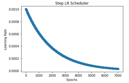
Below, we have again used step LR scheduler but this time we have used it to change the learning rate after each batch. The majority of changes are the same with only changes step lr parameters. For this example, we have set step size to 20 and gamma to 0.99. This will inform the scheduler to decrease learning by a factor of 0.99 after every 20 batches.
We have also plotted a chart showing how the learning rate changes during the training process for explanation purposes.
from torch.optim import SGD, RMSprop, Adam
from torch.optim import lr_scheduler

#torch.manual_seed(42) ##For reproducibility.This will make sure that same random weights are initialized each time.
epochs = 15
learning_rate = torch.tensor(1e-3) # 0.001

conv_net = ConvNet()
cross_entropy_loss = nn.CrossEntropyLoss()
optimizer = SGD(params=conv_net.parameters(), lr=learning_rate)
scheduler = lr_scheduler.StepLR(optimizer, step_size=20, gamma=0.99)

val_acc = TrainModelInBatchesV3(conv_net, cross_entropy_loss, optimizer, [scheduler], train_loader, test_loader,epochs)
scheduler_val_accs["Step LR Scheduler Batches"] = val_acc
import matplotlib.pyplot as plt

conv_net = ConvNet()
optimizer = SGD(params=conv_net.parameters(), lr=learning_rate)
scheduler = lr_scheduler.StepLR(optimizer, step_size=20, gamma=0.99)

lrs = []
for i in range(epochs):
    for j in range(len(train_loader)):
        lrs.append(optimizer.state_dict()["param_groups"][0]["lr"].item())
        optimizer.step()
        scheduler.step()

plt.scatter(range(epochs*len(train_loader)), lrs)
plt.title("Step LR Scheduler")
plt.xlabel("Epochs")
plt.ylabel("Learning Rate");
3. MultiStep LR Scheduler 
In this section, we have trained our network using a multi-step lr scheduler. We can create multi-step LR using MultiStepLR() constructor. It takes a list of the below-mentioned parameters.
- optimizer - The first parameter is an instance of the optimizer.
- milestones - This parameter accepts a list of integers specifying boundaries of epochs till which to apply a particular learning rate and then change it. This will become more clear when we explain it with the example below.
- gamma - This is a float value specifying multiplicative factor.
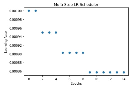
In our case, we have initialized multi-step LR with milestones of [2,5,9] and gamma of 0.95. This will inform the scheduler to use the initial learning rate for the first 2 epochs (0,1) and then reduce the learning rate by a multiplicative factor of 0.95. Then, use reduced learning rate for the next 3 epochs (2,3,4) and reduce the learning rate again by a factor of 0.95. Then use reduced learning rate for the next 4 epochs (5,6,7,8) and reduce the learning rate again by a factor of 0.95. At last, use reduced learning rate for all remaining epochs (9,10,11,12,13,14).
We have also plotted learning rate changes over time in the next cell after training for explanation purposes.
from torch.optim import SGD, RMSprop, Adam
from torch.optim import lr_scheduler

#torch.manual_seed(42) ##For reproducibility.This will make sure that same random weights are initialized each time.
epochs = 15
learning_rate = torch.tensor(1e-3) # 0.001

conv_net = ConvNet()
cross_entropy_loss = nn.CrossEntropyLoss()
optimizer = SGD(params=conv_net.parameters(), lr=learning_rate)
scheduler = lr_scheduler.MultiStepLR(optimizer, milestones=[2,5,9], gamma=0.95)

val_acc = TrainModelInBatchesV2(conv_net, cross_entropy_loss, optimizer, [scheduler], train_loader, test_loader,epochs)
scheduler_val_accs["MultiStep LR Scheduler Epochs"] = val_acc
import matplotlib.pyplot as plt

conv_net = ConvNet()
optimizer = SGD(params=conv_net.parameters(), lr=learning_rate)
scheduler = lr_scheduler.MultiStepLR(optimizer, milestones=[2,5,9], gamma=0.95)

lrs = []
for i in range(epochs):
    lrs.append(optimizer.state_dict()["param_groups"][0]["lr"].item())
    optimizer.step()
    scheduler.step()

plt.scatter(range(epochs), lrs)
plt.title("Multi Step LR Scheduler")
plt.xlabel("Epochs")
plt.ylabel("Learning Rate");
4. Multiplicative LR Scheduler 
In this section, we have trained our network using SGD with a multiplicative learning rate scheduler. We can create a multiplicative LR scheduler using MultiplicativeLR() constructor from lr_scheduler module. It multiplies the learning rate by a specified value after the completion of each epoch to reduce the learning rate. Below are important parameters of the constructor.
- optimizer - We need to provide optimizer object as first parameter.
- lr_lambda - This parameter accepts function that returns multiplication factor for each epoch.
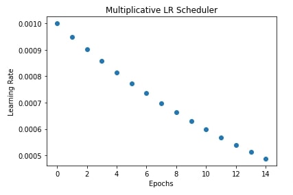
In our case, we have created a multiplicative learning rate scheduler with a function that multiplies the current learning rate by 0.95 after the completion of each epoch to reduce the learning rate.
In the next cell after the training cell, we have also plotted how the learning rate changes during training if we use a multiplicative learning rate scheduler.
from torch.optim import SGD, RMSprop, Adam
from torch.optim import lr_scheduler

#torch.manual_seed(42) ##For reproducibility.This will make sure that same random weights are initialized each time.
epochs = 15
learning_rate = torch.tensor(1e-3) # 0.001

conv_net = ConvNet()
cross_entropy_loss = nn.CrossEntropyLoss()
optimizer = SGD(params=conv_net.parameters(), lr=learning_rate)
scheduler = lr_scheduler.MultiplicativeLR(optimizer, lr_lambda=lambda epoch: 0.95)

val_acc = TrainModelInBatchesV2(conv_net, cross_entropy_loss, optimizer, [scheduler], train_loader, test_loader,epochs)
scheduler_val_accs["Multiplicative LR Scheduler Epochs"] = val_acc
import matplotlib.pyplot as plt

conv_net = ConvNet()
optimizer = SGD(params=conv_net.parameters(), lr=learning_rate)
scheduler = lr_scheduler.MultiplicativeLR(optimizer, lr_lambda=lambda epoch: 0.95)

lrs = []
for i in range(epochs):
    lrs.append(optimizer.state_dict()["param_groups"][0]["lr"].item())
    optimizer.step()
    scheduler.step()


plt.scatter(range(epochs), lrs)
plt.title("Multiplicative LR Scheduler")
plt.xlabel("Epochs")
plt.ylabel("Learning Rate");
5. Lambda LR Scheduler 
In this section, we have trained our network using a lambda learning rate scheduler which sets the learning rate to the initial learning rate times output of a lambda function. We can create a lambda learning rate scheduler using LambdaLR() constructor available from lr_schedule module. Below are important parameters of the constructor.
- optimizer - The first parameter should be an instance of an optimizer.
- lr_lambda - This parameter accepts a function whose output is multiplied with the initial learning rate to generate a new learning rate after each epoch.
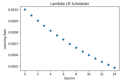
In our case we have initialize LambdaLR() with lambda epoch: 0.95**epoch function. This will multiply the initial learning rate of 0.001 by 0.95**epoch after each epoch where epoch is epoch number.
In the next cell, we have also plotted how the learning rate will change during the training process if we use the lambda learning rate scheduler.
from torch.optim import SGD, RMSprop, Adam
from torch.optim import lr_scheduler

#torch.manual_seed(42) ##For reproducibility.This will make sure that same random weights are initialized each time.
epochs = 15
learning_rate = torch.tensor(1e-3) # 0.001

conv_net = ConvNet()
cross_entropy_loss = nn.CrossEntropyLoss()
optimizer = SGD(params=conv_net.parameters(), lr=learning_rate)
scheduler = lr_scheduler.LambdaLR(optimizer, lambda epoch: 0.95**epoch)

val_acc = TrainModelInBatchesV2(conv_net, cross_entropy_loss, optimizer, [scheduler], train_loader, test_loader,epochs)
scheduler_val_accs["Lambda LR Scheduler Epochs"] = val_acc
import matplotlib.pyplot as plt

conv_net = ConvNet()
optimizer = SGD(params=conv_net.parameters(), lr=learning_rate)
scheduler = lr_scheduler.LambdaLR(optimizer, lambda epoch: 0.95**epoch)

lrs = []
for i in range(epochs):
    lrs.append(optimizer.state_dict()["param_groups"][0]["lr"].item())
    optimizer.step()
    scheduler.step()

plt.scatter(range(epochs), lrs)
plt.title("Lambda LR Scheduler")
plt.xlabel("Epochs")
plt.ylabel("Learning Rate");
6. Exponential LR Scheduler 
In this section, we have trained our network using SGD with an exponential LR scheduler. We can create exponential LR scheduler using ExponentialLR() constructor available from lr_scheduler sub-module. It decays the learning rate exponentially based on the decay rate given as input. Below are important parameters of ExponentialLR() constructor.
- optimizer - The first parameter is an instance of the optimizer.
- gamma - This is a multiplicative factor that will be raised to power based on epoch number and multiplied by the initial learning rate to get a new learning rate.
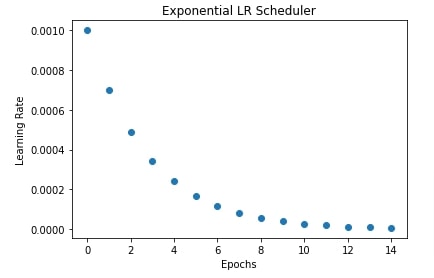
In our case, we have created an exponential LR scheduler with gamma set to 0.7. The initial learning rate is 0.001. The learning rate for first epoch will be 0.001 * gamma ^ 0 = 0.001. For second epoch, it'll be 0.001 * gamma^1 = 0.0007. For the third epoch, it'll be 0.001 * gamma^2 = 0.00049 and so on for upcoming epochs.
In the next cell after training, we have also plotted a chart showing how the learning rate changes over time during training if we use an exponential learning rate scheduler.
from torch.optim import SGD, RMSprop, Adam
from torch.optim import lr_scheduler

#torch.manual_seed(42) ##For reproducibility.This will make sure that same random weights are initialized each time.
epochs = 15
learning_rate = torch.tensor(1e-3) # 0.001

conv_net = ConvNet()
cross_entropy_loss = nn.CrossEntropyLoss()
optimizer = SGD(params=conv_net.parameters(), lr=learning_rate)
scheduler = lr_scheduler.ExponentialLR(optimizer, gamma=0.7)

val_acc = TrainModelInBatchesV2(conv_net, cross_entropy_loss, optimizer, [scheduler], train_loader, test_loader,epochs)
scheduler_val_accs["Exponential LR Scheduler Epochs"] = val_acc
import matplotlib.pyplot as plt

conv_net = ConvNet()
optimizer = SGD(params=conv_net.parameters(), lr=learning_rate)
scheduler = lr_scheduler.ExponentialLR(optimizer, gamma=0.7)

lrs = []
for i in range(epochs):
    lrs.append(optimizer.state_dict()["param_groups"][0]["lr"].item())
    optimizer.step()
    scheduler.step()


plt.scatter(range(epochs), lrs)
plt.title("Exponential LR Scheduler")
plt.xlabel("Epochs")
plt.ylabel("Learning Rate");
7. One Cycle LR Scheduler 
In this section, we have used one cycle LR scheduler to train our network. This LR scheduler changes the learning rate after each batch of data. As the name suggests, it changes the learning rate in cycle mode. It is inspired by the paper - Super-Convergence: Very Fast Training of Neural Networks Using Large Learning Rates. We can create it using OneCycleLR() constructor. Below are important parameters of the constructor.
- optimizer - The first parameter is the optimizer instance as usual.
- max_lr - This is the maximum learning rate that the scheduler should go during the cycle.
- steps_per_epoch - This parameter accepts integer values specifying a total number of batches per epoch.
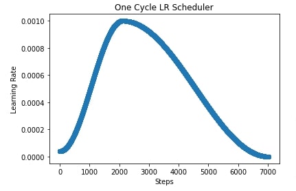
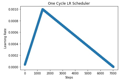
- pct_start - This parameter accepts float value in the range [0,1]. The learning rate increases to the max learning rate after the percentage of batches specified using this parameter has passed. The learning rate then starts decreasing. Default is 0.3 which means that maximum learning rate will be achieved at 30% of batches and then it'll start decreasing.
- anneal_strategy - This parameter accepts one of the below strings specifying how to anneal the learning rate.
- 'linear' - It anneals the learning rate in linear line fashion.
- 'cosine' - It anneals the learning rate in a cosine cycle-like fashion. Default.
- epochs - This parameter accepts integers specifying the number of epochs.
- div_factor - This parameter accepts float value that is used to determine the initial learning rate to start a cycle. The default value is 25.
- Initial learning rate = maximum learning rate / div_factor
- final_div_factor - This parameter accepts float specifying minimum learning rate should go at the end of the cycle. Default value is 1e4.
- minimum learning rate = initial learning rate / final_div_factor
In our case, we have initialized OneCycleLR with a max learning rate of 0.001.
In the next cell, we have plotted how the learning rate changes over time during training. In the cell after that, we have also plotted another learning rate chart where we have shown how learning rate changes if we use 'linear' annealing strategy instead of 'cosine'.
from torch.optim import SGD, RMSprop, Adam
from torch.optim import lr_scheduler

#torch.manual_seed(42) ##For reproducibility.This will make sure that same random weights are initialized each time.
epochs = 15
learning_rate = torch.tensor(1e-3) # 0.001

conv_net = ConvNet()
cross_entropy_loss = nn.CrossEntropyLoss()
optimizer = SGD(params=conv_net.parameters(), lr=learning_rate)
scheduler = lr_scheduler.OneCycleLR(optimizer, max_lr=learning_rate,
                                    steps_per_epoch=len(train_loader), epochs=epochs)

val_acc = TrainModelInBatchesV3(conv_net, cross_entropy_loss, optimizer, [scheduler], train_loader, test_loader,epochs)
scheduler_val_accs["One Cycle LR Scheduler Batches"] = val_acc
import matplotlib.pyplot as plt

conv_net = ConvNet()
optimizer = SGD(params=conv_net.parameters(), lr=learning_rate)
scheduler = lr_scheduler.OneCycleLR(optimizer, max_lr=learning_rate,
                                    steps_per_epoch=len(train_loader), epochs=epochs)

lrs = []
for i in range(epochs):
    for j in range(len(train_loader)):
        lrs.append(optimizer.state_dict()["param_groups"][0]["lr"].item())
        optimizer.step()
        scheduler.step()


plt.scatter(range(epochs*len(train_loader)), lrs)
plt.title("One Cycle LR Scheduler")
plt.xlabel("Steps")
plt.ylabel("Learning Rate");
import matplotlib.pyplot as plt

conv_net = ConvNet()
optimizer = SGD(params=conv_net.parameters(), lr=learning_rate)
scheduler = lr_scheduler.OneCycleLR(optimizer, max_lr=learning_rate,
                                    steps_per_epoch=len(train_loader),
                                    pct_start=0.2, anneal_strategy="linear",epochs=epochs)

lrs = []
for i in range(epochs):
    for j in range(len(train_loader)):
        lrs.append(optimizer.state_dict()["param_groups"][0]["lr"].item())
        optimizer.step()
        scheduler.step()


plt.scatter(range(epochs*len(train_loader)), lrs)
plt.title("One Cycle LR Scheduler")
plt.xlabel("Steps")
plt.ylabel("Learning Rate");
8. Cyclic LR Scheduler 
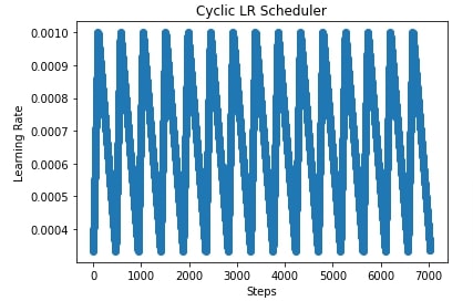
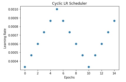
In this section, we have introduced cyclical learning rate schedules which increase and decrease learning in a cyclical fashion during training. It is inspired by the paper - Cyclical Learning Rates for Training Neural Networks. Unlike one cycle LR scheduler from the previous section which has only one cycle, cyclic LR scheduler has many cycles. We can create a cyclic LR scheduler using CyclicLR() constructor. Below are important parameters of CyclicLR() constructor.
- optimizer - The first parameter to the scheduler is the optimizer instance as usual.
- base_lr - This is the minimum learning rate at which the cycle starts.
- max_lr - This is the maximum learning rate of the cycle.
- step_size_up - This parameter accepts integer value specifying for how many batches increase the learning rate to take from base lr to max LR.
- step_size_down - This parameter accepts integer value specifying for how many batches to decrease the learning rate from max LR.
In our case, we have initialized CyclicLR() with a base learning rate that is third of maximum learning rate, step size up of 100, and step size down to total batches minus 100. This will start with the initial learning rate which is a third of the maximum learning rate, it'll reach the maximum learning rate at 100 batches, and then it'll keep decreasing the learning rate till all batches of the data loader are completed. This is considered one cycle. The same cycle will be repeated for all epochs.
In the next cells, we have plotted how learning rate changes during training if we use a cyclic learning rate scheduler.
from torch.optim import SGD, RMSprop, Adam
from torch.optim import lr_scheduler

#torch.manual_seed(42) ##For reproducibility.This will make sure that same random weights are initialized each time.
epochs = 15
learning_rate = torch.tensor(1e-3) # 0.001

conv_net = ConvNet()
cross_entropy_loss = nn.CrossEntropyLoss()
optimizer = SGD(params=conv_net.parameters(), lr=learning_rate)
scheduler = lr_scheduler.CyclicLR(optimizer, base_lr=learning_rate/3,
                                  max_lr=learning_rate, step_size_up=100,
                                  step_size_down=len(train_loader)-100)

val_acc = TrainModelInBatchesV3(conv_net, cross_entropy_loss, optimizer, [scheduler], train_loader, test_loader,epochs)
scheduler_val_accs["Cyclic LR Scheduler Batches"] = val_acc
import matplotlib.pyplot as plt

conv_net = ConvNet()
optimizer = SGD(params=conv_net.parameters(), lr=learning_rate)
scheduler = lr_scheduler.CyclicLR(optimizer, base_lr=learning_rate/3,
                                  max_lr=learning_rate, step_size_up=100,
                                  step_size_down=len(train_loader)-100)

lrs = []
for i in range(epochs):
    for j in range(len(train_loader)):
        lrs.append(optimizer.state_dict()["param_groups"][0]["lr"].item())
        optimizer.step()
        scheduler.step()


plt.scatter(range(epochs*len(train_loader)), lrs)
plt.title("Cyclic LR Scheduler")
plt.xlabel("Steps")
plt.ylabel("Learning Rate");
import matplotlib.pyplot as plt

conv_net = ConvNet()
optimizer = SGD(params=conv_net.parameters(), lr=learning_rate)
scheduler = lr_scheduler.CyclicLR(optimizer, base_lr=learning_rate/3, max_lr=learning_rate, step_size_up=5, step_size_down=None)

lrs = []
for i in range(epochs):
    lrs.append(optimizer.state_dict()["param_groups"][0]["lr"].item())
    optimizer.step()
    scheduler.step()


plt.scatter(range(epochs), lrs)
plt.title("Cyclic LR Scheduler")
plt.xlabel("Epochs")
plt.ylabel("Learning Rate");
9. Cosine Annealing LR Scheduler 
In this section, we have trained our network using SGD with a cosine annealing learning rate scheduler. It is inspired by the paper - SGDR: Stochastic Gradient Descent with Warm Restarts. We can create cosine annealing scheduler using CosineAnnealingLR() constructor available from lr_scheduler sub-module. Below are important parameters of the constructor.
- optimizer - The first parameter is optimizer instance.
- T_max - This parameter accepts integer specifying a maximum number of iterations (epochs/batches) over which to anneal learning rate.
- eta_min - This is the minimum learning rate at the end of T_max iterations.
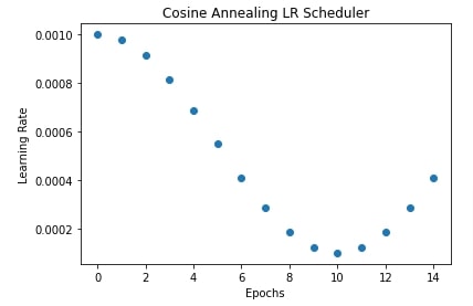
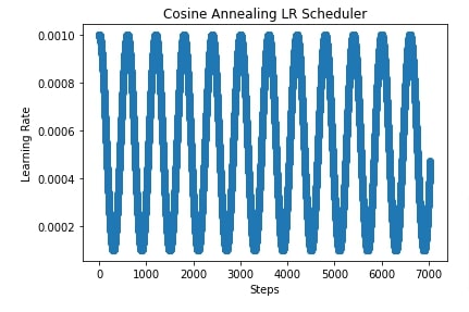
In our case below, we have initialized CosineAnnealingLR() with T_max set to 10 and eta_min set to 0.0001. The learning rate will start with 0.001 and then it'll reduce to 0.0001 in cosine curve fashion. Then it'll increase for T_max iterations and so on. It'll keep on decreasing and increasing for T_max iterations.
In the next cells, we have plotted how the learning rate will change during training if we use a cosine annealing learning rate scheduler to anneal learning rate.
from torch.optim import SGD, RMSprop, Adam
from torch.optim import lr_scheduler

#torch.manual_seed(42) ##For reproducibility.This will make sure that same random weights are initialized each time.
epochs = 15
learning_rate = torch.tensor(1e-3) # 0.001

conv_net = ConvNet()
cross_entropy_loss = nn.CrossEntropyLoss()
optimizer = SGD(params=conv_net.parameters(), lr=learning_rate)
scheduler = lr_scheduler.CosineAnnealingLR(optimizer, T_max=10, eta_min=0.0001)

val_acc = TrainModelInBatchesV2(conv_net, cross_entropy_loss, optimizer, [scheduler], train_loader, test_loader,epochs)
scheduler_val_accs["Cosine Annealing LR Scheduler Epochs"] = val_acc
import matplotlib.pyplot as plt

conv_net = ConvNet()
optimizer = SGD(params=conv_net.parameters(), lr=learning_rate)
scheduler = lr_scheduler.CosineAnnealingLR(optimizer, T_max=10, eta_min=0.0001)

lrs = []
for i in range(epochs):
    lrs.append(optimizer.state_dict()["param_groups"][0]["lr"].item())
    optimizer.step()
    scheduler.step()


plt.scatter(range(epochs), lrs)
plt.title("Cosine Annealing LR Scheduler")
plt.xlabel("Epochs")
plt.ylabel("Learning Rate");
import matplotlib.pyplot as plt

conv_net = ConvNet()
optimizer = SGD(params=conv_net.parameters(), lr=learning_rate)
scheduler = lr_scheduler.CosineAnnealingLR(optimizer, T_max=300, eta_min=0.0001)

lrs = []
for i in range(epochs):
    for j in range(len(train_loader)):
        lrs.append(optimizer.state_dict()["param_groups"][0]["lr"].item())
        optimizer.step()
        scheduler.step()


plt.scatter(range(epochs*len(train_loader)), lrs)
plt.title("Cosine Annealing LR Scheduler")
plt.xlabel("Steps")
plt.ylabel("Learning Rate");
10. Cosine Annealing With Warm Restarts Scheduler 
In this section, we have trained our network using a cosine annealing scheduler with warm restarts. It is inspired by the paper - SGDR: Stochastic Gradient Descent with Warm Restarts. We can create cosine annealing with warm restarts scheduler using CosineAnnealingWarmRestarts() constructor available from lr_scheduler sub-module. Below are important parameters of the constructor.
- optimizer - The first parameter is optimizer instance as usual.
- T_0 - It accepts integer specifying number of iterations (epochs/batches) for first restart (cycle).
- T_mult - This parameter accepts that is used to factor increase cycle iterations.
- eta_min - This parameter specifies minimum learning rate that should go in one cycle.
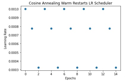
In our case, we have initialized CosineAnnealingWarmRestarts() with T_0 set to 3, T_mult set to 1 and eta_min set to 0.0001. The scheduler will start with an initial learning rate of 0.001 and reduce it to 0.0001 in 3 epochs. Then, it'll start again with a learning rate of 0.001 and decrease it to 0.0001 in 3 epochs.
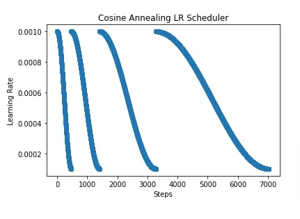
In these next 2 cells, we have plotted a chart showing how the learning rate changes if we use cosine annealing with a warm restarts scheduler.
from torch.optim import SGD, RMSprop, Adam
from torch.optim import lr_scheduler

#torch.manual_seed(42) ##For reproducibility.This will make sure that same random weights are initialized each time.
epochs = 15
learning_rate = torch.tensor(1e-3) # 0.001

conv_net = ConvNet()
cross_entropy_loss = nn.CrossEntropyLoss()
optimizer = SGD(params=conv_net.parameters(), lr=learning_rate)
scheduler = lr_scheduler.CosineAnnealingWarmRestarts(optimizer, T_0=3, T_mult=1, eta_min=0.0001)

val_acc = TrainModelInBatchesV2(conv_net, cross_entropy_loss, optimizer, [scheduler], train_loader, test_loader,epochs)
scheduler_val_accs["Cosine Annealing With Warm Restarts Scheduler Epochs"] = val_acc
import matplotlib.pyplot as plt
conv_net = ConvNet()
optimizer = SGD(params=conv_net.parameters(), lr=learning_rate)
scheduler = lr_scheduler.CosineAnnealingWarmRestarts(optimizer, T_0=3, T_mult=1, eta_min=0.0001)
lrs = []
for i in range(epochs):
lrs.append(optimizer.state_dict()["param_groups"][0]["lr"].item())
optimizer.step()
scheduler.step()
plt.scatter(range(epochs), lrs)
plt.title("Cosine Annealing Warm Restarts LR Scheduler")
plt.xlabel("Epochs")
plt.ylabel("Learning Rate");
import matplotlib.pyplot as plt
conv_net = ConvNet()
optimizer = SGD(params=conv_net.parameters(), lr=learning_rate)
scheduler = lr_scheduler.CosineAnnealingWarmRestarts(optimizer, T_0=len(train_loader), T_mult=2, eta_min=0.0001)
lrs = []
for i in range(epochs):
for j in range(len(train_loader)):
lrs.append(optimizer.state_dict()["param_groups"][0]["lr"].item())
optimizer.step()
scheduler.step()
plt.scatter(range(epochs*len(train_loader)), lrs)
plt.title("Cosine Annealing LR Scheduler")
plt.xlabel("Steps")
plt.ylabel("Learning Rate");
11. Reduce LR On Plateau Scheduler 
In this section, we have introduced another learning rate scheduler that reduces learning rate by monitoring metrics like loss, accuracy, etc. It reduces the learning rate only when the metric it is monitoring is not improving further. We can create reduce LR on the plateau scheduler using ReduceLROnPlateau() constructor. Below are important parameters of the constructor.
- optimizer - The first parameter is the optimizer instance as usual.
- mode - The mode specifies using string whether we want to monitor minimization of value of metric or maximization.
- factor - The factor is the float value by which the current learning rate is multiplied to get a new learning rate if a metric is not improving.
- patience - This parameter accepts integer value specifying for how many constant epochs if metrics are not improving then the learning rate should be changed.
- threshold - This parameter accepts float value specifying at least by how much amount metric should improve.
- min_lr - This is the minimum learning rate. The learning rate won't reduce beyond this.
Below, we have modified our training routine because now we have to provide metrics that we are monitoring in the call of the step() method of scheduler instance. We have asked our scheduler to monitor validation loss.
In our case, we have created a scheduler with an initial learning rate of 0.001, a factor of 0.95, the patience of 3, the threshold of 0.001 and a minimum learning rate of 0.0001. This will start with an initial learning rate of 0.001 and if validation loss is not decreased by at least 0.001 for 3 consecutive epochs then reduce the current learning rate to the current learning rate multiplied by 0.95.
from tqdm import tqdm
def CalcValLoss(model, loss_func, val_loader):
with torch.no_grad(): ## Prevents calculation of gradients
val_losses = []
for X_batch, Y_batch in val_loader:
preds = model(X_batch)
loss = loss_func(preds, Y_batch)
val_losses.append(loss)
val_loss = torch.tensor(val_losses).mean()
print("Valid CategoricalCrossEntropy : {:.3f}".format(val_loss))
return val_loss
def TrainModelInBatchesV4(model, loss_func, optimizer, scheduler, train_loader, val_loader, epochs=5):
for i in range(epochs):
losses = [] ## Record loss of each batch
for X_batch, Y_batch in tqdm(train_loader):
preds = model(X_batch) ## Make Predictions by forward pass through network
loss = loss_func(preds, Y_batch) ## Calculate Loss
losses.append(loss) ## Record Loss
optimizer.zero_grad() ## Zero weights before calculating gradients
loss.backward() ## Calculate Gradients
optimizer.step() ## Update Weights
print("Train CategoricalCrossEntropy : {:.3f}".format(torch.tensor(losses).mean()))
val_loss = CalcValLoss(model, loss_func, val_loader)
scheduler.step(val_loss)
Y_test_shuffled, test_preds = MakePredictions(model, val_loader)
val_acc = accuracy_score(Y_test_shuffled, test_preds)
print("Val Accuracy : {:.3f}".format(val_acc))
return val_acc
from torch.optim import SGD, RMSprop, Adam
from torch.optim import lr_scheduler
#torch.manual_seed(42) ##For reproducibility.This will make sure that same random weights are initialized each time.
epochs = 15
learning_rate = torch.tensor(1e-3) # 0.001
conv_net = ConvNet()
cross_entropy_loss = nn.CrossEntropyLoss()
optimizer = SGD(params=conv_net.parameters(), lr=learning_rate)
scheduler = lr_scheduler.ReduceLROnPlateau(optimizer, mode='min',
factor=0.95, patience=3,
threshold=0.001, min_lr=0.0001, verbose=True)
val_acc = TrainModelInBatchesV4(conv_net, cross_entropy_loss, optimizer, scheduler, train_loader, test_loader,epochs)
scheduler_val_accs["Reduce LR On Plateau Scheduler"] = val_acc
12. Combining Multiple Schedulers 
In this section, we have explained how we can combine multiple schedulers when using PyTorch. As we had said earlier, PyTorch let us execute more than one scheduler to apply the effect of them on learning rate together.
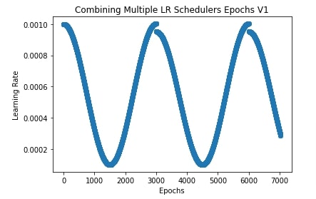
Below, we have created two schedulers that we'll use for our example. We have created a step learning rate scheduler and cosine annealing learning rate schedules. We have given both as a list to our training routine.
In the next cell, we have also plotted how the learning rate will change during training if we apply two schedulers one after another.
from torch.optim import SGD, RMSprop, Adam
from torch.optim import lr_scheduler
#torch.manual_seed(42) ##For reproducibility.This will make sure that same random weights are initialized each time.
epochs = 15
learning_rate = torch.tensor(1e-3) # 0.001
conv_net = ConvNet()
cross_entropy_loss = nn.CrossEntropyLoss()
optimizer = SGD(params=conv_net.parameters(), lr=learning_rate)
scheduler1 = lr_scheduler.StepLR(optimizer, step_size=2, gamma=0.95)
scheduler2 = lr_scheduler.CosineAnnealingLR(optimizer, T_max=10, eta_min=0.0001)
val_acc = TrainModelInBatchesV3(conv_net, cross_entropy_loss, optimizer, [scheduler1, scheduler2], train_loader, test_loader,epochs)
scheduler_val_accs["Combining Multiple LR Schedulers Epochs V1"] = val_acc
import matplotlib.pyplot as plt
conv_net = ConvNet()
optimizer = SGD(params=conv_net.parameters(), lr=learning_rate)
scheduler1 = lr_scheduler.StepLR(optimizer, step_size=1500, gamma=0.95)
scheduler2 = lr_scheduler.CosineAnnealingLR(optimizer, T_max=1500, eta_min=0.0001)
lrs = []
for i in range(epochs):
for j in range(len(train_loader)):
lrs.append(optimizer.state_dict()["param_groups"][0]["lr"].item())
optimizer.step()
scheduler1.step()
scheduler2.step()
plt.scatter(range(epochs* len(train_loader)), lrs)
plt.title("Combining Multiple LR Schedulers Epochs V1")
plt.xlabel("Epochs")
plt.ylabel("Learning Rate");
Below, we have created another example demonstrating the usage of multiple schedulers. We have modified our training routine to use different schedulers based on the number of batches completed. We are passing 4 schedulers to our training routine. The first scheduler is used for 2000 batches at the start. Then for another 2000 batches, the second scheduler is used and the third scheduler for another 2000 batches. The remaining batches at the end are executed with the fourth scheduler.
In the next cell, we have also plotted how the learning rate changes during training if we combine schedules this way.
def TrainModelInBatchesV5(model, loss_func, optimizer, schedulers, train_loader, val_loader, epochs=5):
steps=0
for i in range(epochs):
losses = [] ## Record loss of each batch
for X_batch, Y_batch in tqdm(train_loader):
preds = model(X_batch) ## Make Predictions by forward pass through network
loss = loss_func(preds, Y_batch) ## Calculate Loss
losses.append(loss) ## Record Loss
optimizer.zero_grad() ## Zero weights before calculating gradients
loss.backward() ## Calculate Gradients
optimizer.step() ## Update Weights
steps += 1
if steps < 2000:
schedulers[0].step()
elif steps >= 2000 and steps <= 4000:
schedulers[1].step()
elif steps >= 4000 and steps <= 6000:
schedulers[2].step()
else:
schedulers[3].step()
print("Train CategoricalCrossEntropy : {:.3f}".format(torch.tensor(losses).mean()))
CalcValLoss(model, loss_func, val_loader)
Y_test_shuffled, test_preds = MakePredictions(model, val_loader)
val_acc = accuracy_score(Y_test_shuffled, test_preds)
print("Val Accuracy : {:.3f}".format(val_acc))
return val_acc
from torch.optim import SGD, RMSprop, Adam
from torch.optim import lr_scheduler
#torch.manual_seed(42) ##For reproducibility.This will make sure that same random weights are initialized each time.
epochs = 15
learning_rate = torch.tensor(3e-3)
total_steps = len(train_loader) * epochs
conv_net = ConvNet()
cross_entropy_loss = nn.CrossEntropyLoss()
optimizer = SGD(params=conv_net.parameters(), lr=learning_rate)
scheduler1 = lr_scheduler.CosineAnnealingLR(optimizer, T_max=2000, eta_min=0.002)
scheduler2 = lr_scheduler.CosineAnnealingLR(optimizer, T_max=2000, eta_min=0.001)
scheduler3 = lr_scheduler.CosineAnnealingLR(optimizer, T_max=2000, eta_min=0.0005)
scheduler4 = lr_scheduler.CosineAnnealingLR(optimizer, T_max=1000, eta_min=0.0001)
schedulers = [scheduler1, scheduler2, scheduler3, scheduler4]
val_acc = TrainModelInBatchesV5(conv_net, cross_entropy_loss, optimizer, schedulers, train_loader, test_loader,epochs)
scheduler_val_accs["Combining Multiple LR Schedulers Epochs V2"] = val_acc
import matplotlib.pyplot as plt
conv_net = ConvNet()
optimizer = SGD(params=conv_net.parameters(), lr=learning_rate)
scheduler1 = lr_scheduler.CosineAnnealingLR(optimizer, T_max=2000, eta_min=0.002)
scheduler2 = lr_scheduler.CosineAnnealingLR(optimizer, T_max=2000, eta_min=0.001)
scheduler3 = lr_scheduler.CosineAnnealingLR(optimizer, T_max=2000, eta_min=0.0005)
scheduler4 = lr_scheduler.CosineAnnealingLR(optimizer, T_max=1000, eta_min=0.00001)
schedulers = [scheduler1, scheduler2, scheduler3, scheduler4]
lrs, steps = [], 0
for i in range(epochs):
for j in range(len(train_loader)):
lrs.append(optimizer.state_dict()["param_groups"][0]["lr"])
optimizer.step()
steps += 1
if steps < 2000:
schedulers[0].step()
elif steps >= 2000 and steps <= 4000:
schedulers[1].step()
elif steps >= 4000 and steps <= 6000:
schedulers[2].step()
else:
schedulers[3].step()
plt.scatter(range(epochs*len(train_loader)), lrs)
plt.title("Combining Multiple LR Schedulers Epochs V2")
plt.xlabel("Steps")
plt.ylabel("Learning Rate");

Final Test Set Accuracy Comparison of Various Schedulers 
In this section, we have created a pandas dataframe showing a comparison of the test accuracy of the model with various schedulers. We can notice that schedulers like one cycle and cyclic LR are doing a good job in our case.
import pandas as pd
pd.DataFrame(scheduler_val_accs, index=["Valid Accuracy"]).T
This ends our small tutorial explaining how we can use various learning rate schedulers available from PyTorch. Please feel free to let us know your views in the comments section.
References
 Sunny Solanki
![YouTube Subscribe]() Comfortable Learning through Video Tutorials?
Comfortable Learning through Video Tutorials?
If you are more comfortable learning through video tutorials then we would recommend that you subscribe to our YouTube channel.
![Need Help]() Stuck Somewhere? Need Help with Coding? Have Doubts About the Topic/Code?
Stuck Somewhere? Need Help with Coding? Have Doubts About the Topic/Code?
When going through coding examples, it's quite common to have doubts and errors.
If you have doubts about some code examples or are stuck somewhere when trying our code, send us an email at coderzcolumn07@gmail.com. We'll help you or point you in the direction where you can find a solution to your problem.
You can even send us a mail if you are trying something new and need guidance regarding coding. We'll try to respond as soon as possible.
![Share Views]() Want to Share Your Views? Have Any Suggestions?
Want to Share Your Views? Have Any Suggestions?
If you want to
- provide some suggestions on topic
- share your views
- include some details in tutorial
- suggest some new topics on which we should create tutorials/blogs


 Comfortable Learning through Video Tutorials?
 Stuck Somewhere? Need Help with Coding? Have Doubts About the Topic/Code?
 Want to Share Your Views? Have Any Suggestions?
 pytorch, learning-rate-schedulers