Unsupervised Learning - Clustering
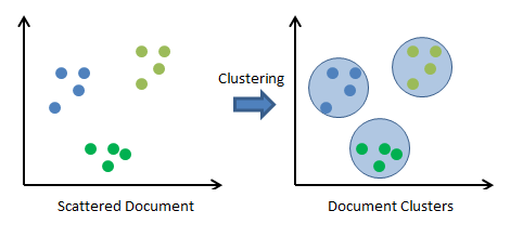
Clustering is a type of Unsupervised Machine Learning. In clustering, developers are not provided any prior knowledge about data like supervised learning where developer knows target variable.
Clustering is the task of creating clusters of samples that have the same characteristics based on some predefined similarity or dissimilarity distance measures like euclidean distance.
Applications of clustering
- Clustering students from class who have the same performance using grades and other attributes for customizing coaching later on.
- Clustering documents together which have content on same topics
- Separating voice from different sources from mixed voice.
- & many more.
Unsupervised Learning Workflow

sklearn.cluster module provides a list of clustering algorithms which we'll try below. We'll start with KMeans and then explore other algorithms.
import numpy as np
import pandas as pd

import matplotlib.pyplot as plt

import sklearn
from sklearn import cluster, datasets

import warnings
import sys

print("Python Version : ",sys.version)
print("Scikit-Learn Version : ",sklearn.__version__)

warnings.filterwarnings('ignore') ## We'll silent future warnings using this command.
np.set_printoptions(precision=3)

## Beow magic function fits plot inside of current notebook.
## There is another option to it (%matplotlib notebook) which opens plot in new notebook.
%matplotlib inline
KMeans
KMeans is an iterative algorithm that begins with random cluster centers and then tries to minimize the distance between sample points and these cluster centers. We need to provide number of clusters in advance. KMeans uses Euclidean distance to measure the distance between cluster centers and sample points. Sample points are moved between clusters if later on, it found that sample points are nearer to some other cluster.
Clustering Example
Dataset Creation
We'll create a dataset with 250 samples, 2 features and 5 cluster centers using scikit-learn's make_blobs method.
samples, clusters = datasets.make_blobs(n_samples=250, n_features=2, centers=5, cluster_std=0.7, random_state=12345)
print('Dataset size : ', samples.shape, clusters.shape)
print('Cluster names : ',set(clusters))
Visualizing Dataset
We'll be visualizing the dataset by plotting scatter chart of Feature-1 and Feature-2. We'll also color-encode and marker-encode each of cluster to show them different.
with plt.style.context(('ggplot', 'seaborn')):
    plt.figure(figsize=(8,6))
    for i, c, m in zip(range(5),['red','green','blue','orange','purple'], ['s','+','^','o', 'x']):
        plt.scatter(samples[clusters == i,0],samples[clusters == i,1], color=c, marker=m, s=80, alpha = 0.8, label= 'Cluster %d'%i)

    plt.xlabel('Feature 1')
    plt.ylabel('Feature 2')
    plt.title('Visualizing Dataset')
    plt.legend(loc='best');

Initializing & Fitting Model
We are initializing KMeans clustering algorithms below with n_clusters=5 because we already know a number of clusters beforehand. For cases where we don't know a number of clusters upfront, we have explained the elbow method below to find out the proper number of clusters.
kmeans = cluster.KMeans(n_clusters=5)
kmeans.fit(samples)
Making Predictions
preds = kmeans.predict(samples)
Calculate Accuracy
We are printing below the accuracy and confusion matrix. We can notice from the confusion matrix that classes returned by kmeans is different from actual classes hence we are getting low accuracy. We need to use the adjusted_rand_score method to handle such scenarios.
from sklearn.metrics import accuracy_score, confusion_matrix, adjusted_rand_score

print('Accuracy : %.3f'%accuracy_score(y_true = clusters, y_pred=preds))
print('Confusion Matrix : \n', confusion_matrix(y_true=clusters, y_pred=preds))
print('Adjusted Accuracy : %.3f'%adjusted_rand_score(labels_true=clusters, labels_pred=preds))
We can also access cluster center for each cluster using cluster_centers_ attribute of KMeans object.
print('Cluster Centers : \n', str(kmeans.cluster_centers_))
We can also access sum of squared distance of each sample from their closest cluster center using intertia_ attribute of KMeans object. It should be as minimum as possible.
print('Sum of squared distances of samples to their closest cluster center : %.2f'%kmeans.inertia_,)
Plotting Cluster Centers & Predictions
Below we are plotting all points of sample data and also linking them to their cluster center using line plot.
with plt.style.context(('ggplot', 'seaborn')):
    plt.figure(figsize=(10,6))

    plt.scatter(samples[preds == 0,0],samples[preds == 0,1], color='red', marker='s', s=80, alpha = 0.8, label= 'Cluster 0')
    plt.scatter(samples[preds == 1,0],samples[preds == 1,1], color='green', marker='^', s=80, alpha = 0.8, label= 'Cluster 1')
    plt.scatter(samples[preds == 2,0],samples[preds == 2,1], color='blue', marker='*', s=80, alpha = 0.8, label= 'Cluster 2')
    plt.scatter(samples[preds == 3,0],samples[preds == 3,1], color='orange', marker='o', s=80, alpha = 0.8, label= 'Cluster 3')
    plt.scatter(samples[preds == 4,0],samples[preds == 4,1], color='purple', marker='+', s=80, alpha = 0.8, label= 'Cluster 4')

    for x,y in zip(samples[preds == 0,0],samples[preds == 0,1]):
        plt.plot([kmeans.cluster_centers_[0][0],x],[kmeans.cluster_centers_[0][1],y], color='red')
    for x,y in zip(samples[preds == 1,0],samples[preds == 1,1]):
        plt.plot([kmeans.cluster_centers_[1][0],x],[kmeans.cluster_centers_[1][1],y], color='green')
    for x,y in zip(samples[preds == 2,0],samples[preds == 2,1]):
        plt.plot([kmeans.cluster_centers_[2][0],x],[kmeans.cluster_centers_[2][1],y], color='blue')
    for x,y in zip(samples[preds == 3,0],samples[preds == 3,1]):
        plt.plot([kmeans.cluster_centers_[3][0],x],[kmeans.cluster_centers_[3][1],y], color='orange')
    for x,y in zip(samples[preds == 4,0],samples[preds == 4,1]):
        plt.plot([kmeans.cluster_centers_[4][0],x],[kmeans.cluster_centers_[4][1],y], color='purple')

    plt.xlabel('Feature 1')
    plt.ylabel('Feature 2')
    plt.title('Visualizing Predictions & Cluster Centers')
    plt.legend(loc='best');

How to decide a number of clusters?
In the above scenario, we already knew a number of clusters in advance. But what if we encounter data for which we aren't aware of a number of possible clusters. There is a method called Elbow method which can be used to solve this problem.
The Elbow Method
Here we look at cluster dispersion for different values of k and plot it. Once plotted we take k value which is at "pit of the elbow" to be a number of clusters. It's based on the intuition that after that many clusters adding more clusters is not improving the sum of squared distances of samples from their clusters further hence that's the best number of clusters one should try.
plt.figure(figsize=(8,5))
distortions = []
for i in range(1,11):
    kmeans = cluster.KMeans(n_clusters=i)
    kmeans.fit(samples)
    distortions.append(kmeans.inertia_)

print('Distortions (Sum Of Squared Distance of Samples from Closest Cluster Center) : ',distortions)

with plt.style.context(('ggplot', 'seaborn')):
    plt.plot(range(1,11), distortions, )
    plt.scatter(range(1,11), distortions, color='red', marker='o', s=80)
    plt.xlabel('Number Of Clusters')
    plt.ylabel('Distortions')
    plt.title('The Elbow Method (Num of Clusters vs Distortions)')
    plt.xticks(range(1,11));

Clustering comes with assumptions: A clustering algorithm finds clusters by making assumptions on how samples should be grouped together. Each algorithm has different assumptions. The quality and interpretability of resulting clusters depend on how these assumptions are satisfied with your goal. For K-means clustering, the model is that all clusters have equal, spherical variance.
 Sunny Solanki
Sunny Solanki
Intro: Software Developer | Youtuber | Bonsai Enthusiast
About: Sunny Solanki holds a bachelor's degree in Information Technology (2006-2010) from L.D. College of Engineering. Post completion of his graduation, he has 8.5+ years of experience (2011-2019) in the IT Industry (TCS). His IT experience involves working on Python & Java Projects with US/Canada banking clients. Since 2020, he’s primarily concentrating on growing CoderzColumn.
His main areas of interest are AI, Machine Learning, Data Visualization, and Concurrent Programming. He has good hands-on with Python and its ecosystem libraries.
Apart from his tech life, he prefers reading biographies and autobiographies. And yes, he spends his leisure time taking care of his plants and a few pre-Bonsai trees.
Contact: sunny.2309@yahoo.in


![YouTube Subscribe]() Comfortable Learning through Video Tutorials?
Comfortable Learning through Video Tutorials?
If you are more comfortable learning through video tutorials then we would recommend that you subscribe to our YouTube channel.
![Need Help]() Stuck Somewhere? Need Help with Coding? Have Doubts About the Topic/Code?
Stuck Somewhere? Need Help with Coding? Have Doubts About the Topic/Code?
 Stuck Somewhere? Need Help with Coding? Have Doubts About the Topic/Code?
When going through coding examples, it's quite common to have doubts and errors.
If you have doubts about some code examples or are stuck somewhere when trying our code, send us an email at coderzcolumn07@gmail.com. We'll help you or point you in the direction where you can find a solution to your problem.
You can even send us a mail if you are trying something new and need guidance regarding coding. We'll try to respond as soon as possible.
![Share Views]() Want to Share Your Views? Have Any Suggestions?
Want to Share Your Views? Have Any Suggestions?
 Want to Share Your Views? Have Any Suggestions?
If you want to
- provide some suggestions on topic
- share your views
- include some details in tutorial
- suggest some new topics on which we should create tutorials/blogs
 clustering, kmeans, unsupervised-learning